
Most of the people while learning data science jump directly into applying the ARIMA or LSTMs when they started learning “time series.” They fit a model, get confusing results, and wonder why. The reason is almost always the same: they skipped the fundamentals.
This post is everything you need to understand before you touch a single model. What makes time series data different, how to read it, what the key concepts mean, and how to prepare it properly. Get this right and every model you build afterward will make more sense.
Regular ML Data vs Time Series Data
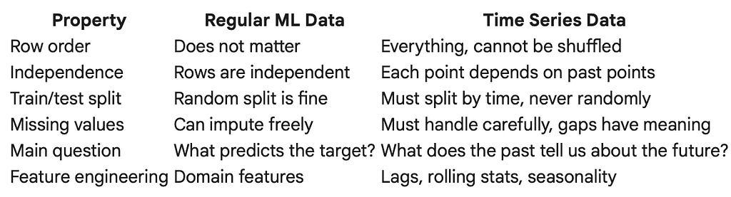
Before anything else, it is worth understanding why time series data needs its own treatment.
In a regular machine learning problem, each row in your dataset is independent. A customer’s purchase record does not depend on the record above it. A patient’s test result does not affect the next patient. You can shuffle the rows and the model still learns the same thing.
Time series data is fundamentally different. Each observation depends on the ones before it. Yesterday’s temperature influences today’s. Last month’s sales affect this month’s inventory. The order of the data is not just a detail, it is the entire point.
A simple example to make this concrete. Suppose you have daily electricity consumption for a city over two years.
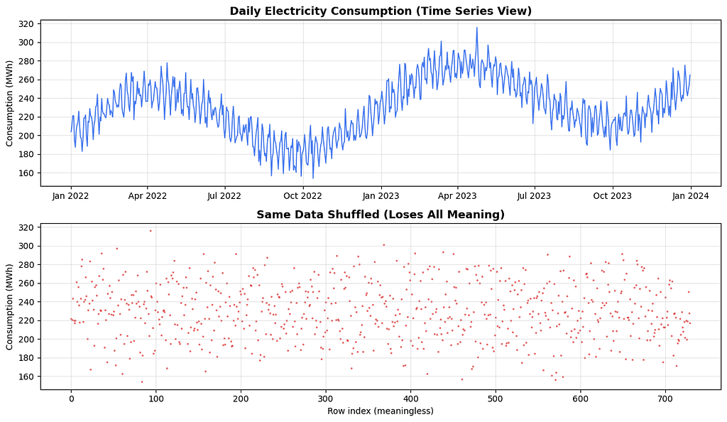
The top chart tells a story: rising trend, annual seasonality, weekly patterns.
The bottom chart is the same numbers shuffled. It is meaningless.
This is why you never randomly shuffle time series data, and never do a random train/test split on it.
Types of Time Series Data
Not all time series behave the same way. Understanding the type you are dealing with shapes every decision afterward.
1. Univariate Time Series
One variable tracked over time. The simplest and most common type.
Examples: daily closing price of a stock, monthly rainfall in Kathmandu, hourly website traffic, weekly product sales.

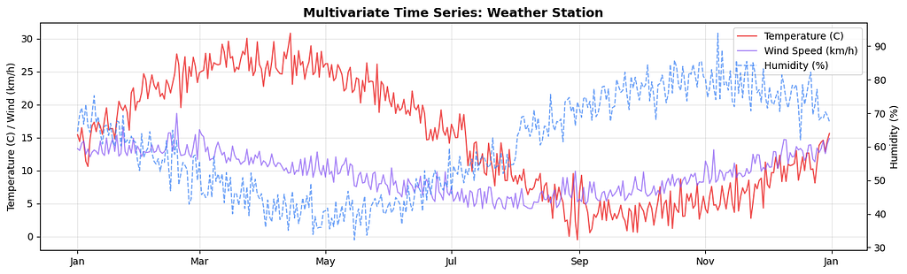
2. Multivariate Time Series
Multiple variables tracked over the same time period, where the variables influence each other.
Examples: temperature, humidity, and wind speed recorded together; a patient’s heart rate, blood pressure, and oxygen saturation over time; a country’s GDP, inflation, and unemployment tracked monthly.
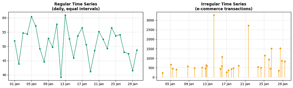
3. Regular vs Irregular Time Series
A regular time series has observations at equal, fixed intervals: every hour, every day, every month.
An irregular time series has observations at uneven intervals: timestamps of customer transactions, timestamps of sensor alerts, timestamps of earthquakes.
4. Continuous vs Discrete Time Series
A continuous time series records values at every instant in theory, like a temperature sensor streaming data. A discrete time series records values only at specific points, like daily closing prices or monthly reports.
In practice, nearly all the time series you will work with in data science are discrete.
Core Terminologies
Before going further, these are the terms you will encounter constantly. Understanding them properly will save a lot of confusion.
Trend
The long-term direction of the series. Is it moving up, down, or staying flat over a long period?
Seasonality
A regular, repeating pattern tied to a fixed calendar period: higher sales every December, higher electricity use every summer, more hospital admissions every flu season. The key word is *fixed period*. Seasonality repeats at the same interval every cycle.
Cyclicality
Similar to seasonality but without a fixed period. Economic cycles, for example, go through expansion and recession roughly every few years, but not on a precise schedule.
The difference matters: seasonality has a known, predictable period; cyclicality does not.
Noise (Residual / Irregular Component)
The random variation left over after you remove trend, seasonality, and cycles. It cannot be predicted. Every real time series has some noise.
Lag
A lag is an earlier version of the series used as a predictor. Lag 1 means yesterday’s value, lag 7 means the value from one week ago, lag 30 means last month’s value. Lag variables are the most fundamental feature engineering technique in time series.

Stationarity: The Most Important Concept in Time Series
Almost every classical time series model, ARIMA, VAR, SARIMA, assumes the data is stationary. If your data is not stationary and you ignore it, your model will give you misleading results. This is the single most common mistake beginners make.
What is Stationarity?
A time series is stationary when its statistical properties do not change over time. Specifically, three things need to be constant:
1. Mean: the average value of the series does not trend up or down.
2. Variance: the spread or volatility of the series stays roughly the same throughout.
3. Auto-covariance: the relationship between the series and its lagged versions does not depend on when you measure it.

Where Does Non-Stationarity Come From?
Non-stationarity is not a flaw in your data. It is the natural state of almost every real-world time series. Here are the most common causes:
- Upward or downward trends: stock prices, population, inflation, product adoption. All of these naturally drift in one direction.
- Seasonality: retail sales spiking every December, restaurant orders spiking on weekends, electricity use peaking in summer.
- Structural breaks: a sudden event changes the behavior of the series permanently. A government regulation, a pandemic, a product launch.
- Changing variance: financial returns are calm during stable periods and volatile during crises. The mean might be stationary but the variance explodes.
Testing for Stationarity:
The Augmented Dickey-Fuller (ADF) test is the standard way to check stationarity statistically. The null hypothesis is that the series is non-stationary (has a unit root). If the p-value is below 0.05, you reject the null and conclude the series is stationary.
How to Make a Non-Stationary Series Stationary
Once you know your series is non-stationary, you need to fix it before modelling. There are several techniques and the right one depends on why the series is non-stationary.
A. Differencing:
Differencing replaces each value with the difference between it and the previous value. It removes trends effectively.
- First-order differencing:
`y’(t) = y(t) — y(t-1)`
2. Second-order differencing: apply differencing twice, useful for strong polynomial trends.
3. Seasonal differencing: subtract the value from the same period in the previous cycle.
`y’(t) = y(t) — y(t — seasonal_period)`

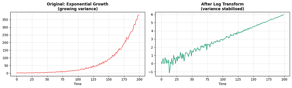
B. Log Transformation:
When the series has exponential growth or growing variance (the volatility increases as the level increases), a log transform compresses the scale and stabilises variance.
C. Detrending:
You can explicitly fit and remove a trend. For a linear trend you fit a regression line and subtract it. For a more complex trend you use techniques like Hodrick-Prescott filtering or STL decomposition.

Rolling Average (Moving Average)
A rolling average, also called a moving average, computes the average of the last N observations at each point in time. It smooths out short-term fluctuations and makes the underlying trend easier to see.
The parameter N is called the window size. A small window follows the original data closely and captures more noise. A large window is smoother but reacts more slowly to real changes.
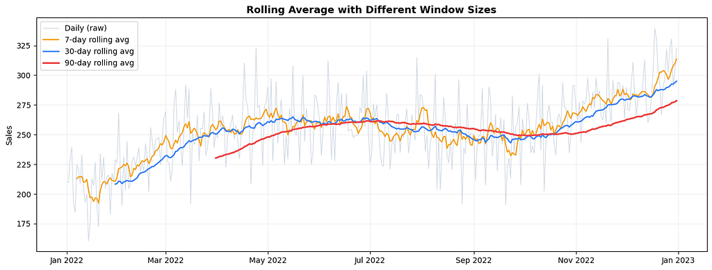
Notice how the 7-day average still shows weekly wobble, the 30-day average reveals the monthly rhythm, and the 90-day average shows only the broad annual trend. Which one you use depends on what you are trying to see.
Rolling averages also have a practical use beyond visualisation: they are features. Rolling mean, rolling standard deviation, and rolling maximum over the last 7 or 30 periods are some of the most useful features you can build for a time series prediction model.
Smoothing and Its Types
Smoothing is the broader family of techniques that rolling average belongs to. Each method handles recent vs older data differently.
Simple Moving Average (SMA)
Gives equal weight to all observations in the window.
SMA(t) = (y(t) + y(t-1) + … + y(t-n+1)) / n
Easy to understand, but old data counts as much as recent data, which is often not ideal.
Weighted Moving Average (WMA)
Gives more weight to recent observations. You define the weights manually.
def weighted_moving_average(series, weights):
    weights = np.array(weights)
    weights = weights / weights.sum()
    result = np.convolve(series, weights[::-1], mode='valid')
    return pd.Series(result, index=series.index[len(weights)-1:])
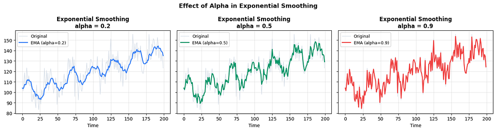
Exponential Smoothing (EWM / EMA)
The most widely used smoothing method. Instead of a fixed window, it applies exponentially decreasing weights to all past observations. The most recent value gets the most weight, and the weight decays exponentially for older values.
The smoothing parameter alpha (between 0 and 1) controls how fast the weights decay.
- High alpha (close to 1): reacts quickly to recent changes, less smooth
- Low alpha (close to 0): reacts slowly, very smooth, follows the long-term level
Holt’s Double Exponential Smoothing
Simple exponential smoothing is great for series with no clear trend. But when there is a trend, it consistently lags behind. Holt’s method adds a second smoothing equation specifically for the trend component.
Two parameters: alpha for the level and beta for the trend.
Holt-Winters Triple Exponential Smoothing
Adds a third smoothing equation for seasonality. This is the most complete of the classical smoothing methods, handling level, trend, and seasonality simultaneously.

Autoregression: The Idea That the Past Predicts the Future
Autoregression is the foundation of most classical time series models. The idea is simple: use the past values of the series itself as predictors.
In regular linear regression you predict y using external features x1, x2, x3. In autoregression you predict y(t) using y(t-1), y(t-2), y(t-3) and so on.
AR(p) means an autoregressive model of order p, using the last p observations as predictors.
y(t) = c + phi_1 * y(t-1) + phi_2 * y(t-2) + … + phi_p * y(t-p) + error

The scatter plots show the key insight:
the correlation between y(t) and y(t-1) is strong,
but
between y(t) and y(t-5) it is much weaker.
This decaying relationship is exactly what the ACF and PACF will show you more rigorously.
Log Transformation in Time Series
The log transformation deserves its own section because it comes up so often and for very specific reasons.
When you see a time series with exponential growth, the series doubles every fixed number of periods. The absolute changes keep getting larger. A 10% growth on a value of 100 is 10, but on a value of 10,000 it is 1,000. This growing variance violates stationarity and makes modelling harder.
Taking the log compresses the scale. It converts multiplicative relationships into additive ones, turns exponential growth into linear growth, and stabilises variance.
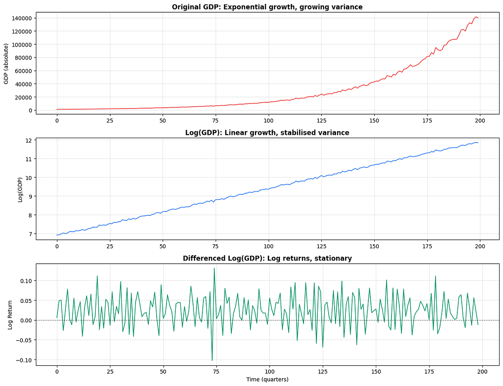
The differenced log series gives you log returns, which is the percentage change between periods. This is the standard representation used in financial time series modelling.
Autocorrelation Function (ACF)
The ACF measures the correlation between the series and each of its lagged versions.
ACF at lag k = correlation between y(t) and y(t-k)
If ACF at lag 1 is 0.8, it means today’s value is strongly correlated with yesterday’s. If ACF at lag 7 is 0.6 in daily data, there is a weekly pattern.
Partial Autocorrelation Function (PACF)
The PACF measures the correlation between y(t) and y(t-k) after removing the effect of all intermediate lags. In other words, it shows the direct relationship between two time points without the influence of the lags in between.
This distinction matters a lot. In an AR(2) process, y(t) depends directly on y(t-1) and y(t-2). But because y(t-1) is also correlated with y(t-2), the ACF shows correlations at many lags even though the direct relationship only goes back two steps. The PACF cuts through this and shows only the direct links.

Now let us see how the pattern changes for an MA process and for seasonal data:

How to Read ACF and PACF: A Summary
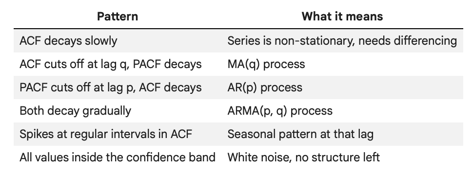
The confidence bands in the plot (the shaded blue region) represent the threshold below which autocorrelations are not statistically significant. Bars that exceed the band are meaningful; bars inside it are essentially noise.
What Comes Next
This post covered everything you need to know before fitting a single model:
- We started with why time series data is different from regular ML data and why order matters.
- We looked at the main types of time series: univariate, multivariate, regular, and irregular.
- We went through the core terminology: trend, seasonality, cyclicality, lag, and the difference between additive and multiplicative structure.
- We covered stationarity in depth, how to test for it with the ADF test, and three methods to fix non-stationarity: differencing, log transforms, and detrending.
- We covered rolling averages and the smoothing family from simple moving averages through to Holt-Winters.
- We unpacked autoregression and why past values are the most natural predictors of future values.
- And finally we covered ACF and PACF, the two diagnostic plots that guide almost every classical model-building decision.
The next post in this series covers the models themselves: ARIMA, SARIMA, and how the concepts from this post translate directly into model parameters.
Thanks for reading up-to this. Will see you next time. & Please don’t forget to clap :) .
Series: Practical Time Series Analysis | Article 01 of Many
GitHub: SujanSB | Medium: sujansb
Note* written with my own old teaching content + cloude.
Time Series Analysis: A Complete Beginner’s Guide Before You Touch Any Model was originally published in Towards AI on Medium, where people are continuing the conversation by highlighting and responding to this story.