Phonons refer to collective vibrational modes in crystals, propagating through the lattice as a wave.
Introduction
One of the most pressing questions in AI research is how language models represent meaning. How does a model know that "excellent" is better than "good"? How does a model represent time scales, e.g., hour vs. day? Where does the knowledge live that July comes after June? Language models are trained to predict text, and they are very good at doing so, but our understanding of their internal representations remains limited. Figuring this out is the holy grail of mechanistic interpretability: the quest of opening the black box and understanding what is going on inside.
There is now growing evidence that semantics are not stored as arbitrary, unstructured patterns. Instead, we find that models encode meaning in predictable geometric structures. A recent example comes from Karkada et al. (2026), who showed that the twelve months of the year form a near-perfect circle in the activation space of a language model (Gemma 2B). The months are not just close to each other in some vague sense, but are arranged in an ordered loop, reflecting the cyclical structure of the year. The question is whether this result is a coincidence, or reflecting something deeper.
Without noting it explicitly, what the authors did in their paper is actually to apply mathematical frameworks established decades ago in the field of solid-state physics, in particular for the study of phonon modes. Phonons describe how vibrations propagate through crystals, and the mathematics behind them provides a rich framework for understanding collective behavior on discrete lattices. The case of the months of the year is an example of one of the simplest structures one can deal with: periodic boundary conditions, where the first and last atom of the chain are coupled to each other, as if bending the chain into a ring. Crucially, physics offers an entire arsenal of further-reaching tools, covering different boundary conditions and higher-dimensional lattice geometries. If the geometry of something like the months of the year can be described through this lens, there is a chance to derive significantly more semantic structure from the same principles. In this post, I lay out the core ideas and share early experimental results for four different boundary condition types.
Background
What are phonons?
A crystal is not a static object. Every atom sits in a potential well created by its neighbors, and at any nonzero temperature, these atoms vibrate. The vibrations do not happen independently: since the atoms are coupled, a disturbance at one site propagates through the lattice as a wave. These collective vibrational modes are called phonons. The insight is that even though the underlying system is a discrete lattice of atoms, the collective behavior can be described by smooth wave functions. A phonon with wavevector
Mapping to AI internals
In the phonon picture, the "atoms" of the lattice are words or tokens, and their positions in the embedding space play the role of atomic displacements. A semantic concept like "levels of quality" defines a one-dimensional chain of tokens ordered by meaning: worst, bad, mediocre, okay, good, excellent, best. The embedding vectors of these tokens are the "displacements" of the atoms.
The mathematical justification for this starts with an "old" result in natural language processing. Word embedding models like word2vec and GloVe learn a word embedding matrix
where
For words that lie on a semantic continuum, the PMI matrix has additional structure. In the absence of other strongly discriminating features, no particular position on the continuum is special, so the co-occurrence probability between two words tends to depend only on their positions along that continuum:
To see what this implies geometrically, consider the eigendecomposition
This means that the
Why is that?
The Gram matrix of the embeddings satisfies
The last equality is exact only if
Geometrically, this means the following: Each word
The eigenvectors
A natural follow-up question is whether this connection carries over to modern language models, which are far more complex than word2vec or GloVe. Recent work suggests that it does, at least as a first approximation. Cagnetta and Wyart (2024) showed that transformers trained on hierarchical data first learn to exploit short-range token correlations before progressively resolving longer-range ones, effectively building deeper representations of the data structure as the training set grows. Complementarily, Rende et al. (2024) demonstrated that transformers learn many-body token interactions in order of increasing degree, with pairwise co-occurrence statistics of the kind captured by PMI being acquired first. This learning hierarchy suggests that the PMI geometry forms a kind of scaffold on which richer representations are later built. Empirical validation for this picture was recently provided by Karkada et al., who showed that PMI-derived geometric predictions persist in the internal activations of Gemma 2B. The spectral structure of co-occurrence is not just an artifact of shallow embedding models; it appears to be a feature that survives into the deeper layers of modern architectures.
The phonon framework gives a physical interpretation to this spectral structure. A phonon mode corresponds to a direction in embedding space along which tokens are coherently displaced, and that direction is precisely one of the eigenmodes of the co-occurrence matrix. If the tokens are arranged according to a smooth vibrational mode
Boundary conditions

Different boundary conditions. Karkada et al. have used periodic boundary conditions for the circular structure of months of the year. Different semantic concepts can be represented by alternative boundary conditions.
Different boundary conditions impose different constraints on how vibrations can look at the endpoints of a chain, and each produces a characteristic geometric signature. The starting point is always the same: we look for modes satisfying
which has the general solution
Periodic boundary conditions
The simplest case is periodic boundary conditions, which connect the two endpoints of the chain as if bending it into a loop. The conditions
whose real and imaginary parts give
Dirichlet boundary conditions
Dirichlet boundary conditions pin the displacement to zero at both endpoints:
The endpoint tokens have zero projection onto every mode. Semantically, this may be interpreted such that the end tokens do not carry any semantic variation, and all representational "richness" lives in the interior of the chain. This might apply to concepts where the extremes are absolute states, something like a scale from "dead" to "alive", where the endpoints are definitionally fixed and the semantic nuance (dying, recovering, thriving…) lives in between.
Neumann boundary conditions
Neumann boundary conditions require the derivative to vanish at both endpoints:
Note that
which is a parabola in the
Robin boundary conditions
Robin boundary conditions interpolate between Dirichlet and Neumann. The condition
Applying the condition at
Note that the Robin BC is not just a theoretical interpolation. Karkada et al. show that for an exponential co-occurrence kernel
2D Neumann boundary conditions
Many semantic concepts are not one-dimensional. When tokens vary along two independent semantic axes, the appropriate framework is a two-dimensional domain with Neumann conditions on all four edges:
The lowest nontrivial modes are
First experiments
I tested this framework with a few boundary conditions at specific semantic concepts, and compared the theoretical prediction to the representations I found in GloVe and in Gemma 2B.
Experimental details
Embedding models: We extract representations from two embedding sources. For GloVe, we use the 300-dimensional GloVe-Wiki-Gigaword embeddings (top 400k vocabulary) loaded via gensim; each concept word is looked up directly and its 300-dimensional vector extracted. Note that the theory holds exactly only in the full-rank regime, where the embedding dimension d is at least as large as the rank of The temperature feels {word} for the temperature scale, The month of the year is {month}, or The amount of storage is one {word} for data-storage units. Activations are extracted using last-token pooling: for each prompt, the hidden-state vector at the final non-padding token position is taken as the representation (the last token aggregates information from the full prompt context).
PCA and geometric fitting: For each concept scale, the
The geometric fit appropriate to each boundary condition type is then applied:
- Periodic BC: For each pair of PCs and each harmonic mode
- Neumann BC: For each pair of PCs, a rotation-agnostic parabola fit is performed: a coarse angular grid search (180 angles over
- Log scale: For each mode
All three fitting procedures incorporate iterative sigma-clipping (threshold
Layer selection for LLM: For Gemma 2B, we perform a layer sweep across layers 1–18 (excluding the raw embedding layer 0). Shown is always the layer of highest
Periodic concepts
I started by validating the result of Karkada et al. and extending it to further cyclic concepts. Besides the months of the year, I tested days of the week and compass directions (north, northeast, east, ...).
Periodic boundary conditions connect the endpoints of the chain into a loop. The resulting modes are complex exponentials, and the first two principal components trace out a circle.
For all three concepts, the tokens arrange themselves in approximately circular structures, though with varying degrees of accuracy. In GloVe, the circular geometry is noisy: the months form a loose arc rather than a clean circle, and the sequential ordering is largely lost. The days of the week are not really circular in structure either, but the compass directions perform quite well. This is interesting, since the word2vec results reported by Karkada et al. for months were considerably cleaner, suggesting that the circular structure is more clearly expressed in some embedding models than others. This is related to the full-rank regime argument: at

Experimental validation of periodic boundary conditions for months of the year, days of the week, and compass directions. In GloVe, the circular structure is noisy and the ordering often scrambled, particularly for months (
Ordinal scales
The next case tests Neumann boundary conditions on three ordinal concepts: levels of quality (terrible to outstanding), temperature (cold to boiling), and emotional valence (devastated to ecstatic), which are examples of open-ended ordinal scales. The tokens have a clear linear ordering, but neither endpoint is pinned to an absolute, immovable value. The rate of semantic change flattens out at the extremes: the difference between "terrible" and "bad" feels smaller than the difference between "terrible" and "decent". I treated this as a signature of Neumann boundary conditions, where the derivative of the mode vanishes at the endpoints. The meaning does not stop abruptly, but it levels off.
The theoretical setup is rather straightforward. Given

The Neumann boundary condition applies to open-ended ordinal scales: concepts with a natural ordering where neither endpoint is semantically pinned to a fixed value. Theory predicts the embeddings to lie on a parabola.
For all three concepts, both in GloVe and Gemma 2B, the embeddings do fall on the predicted parabolic shape. But the parabola does not always appear in the leading two principal components; in several cases it is found in higher-order PCs, such as
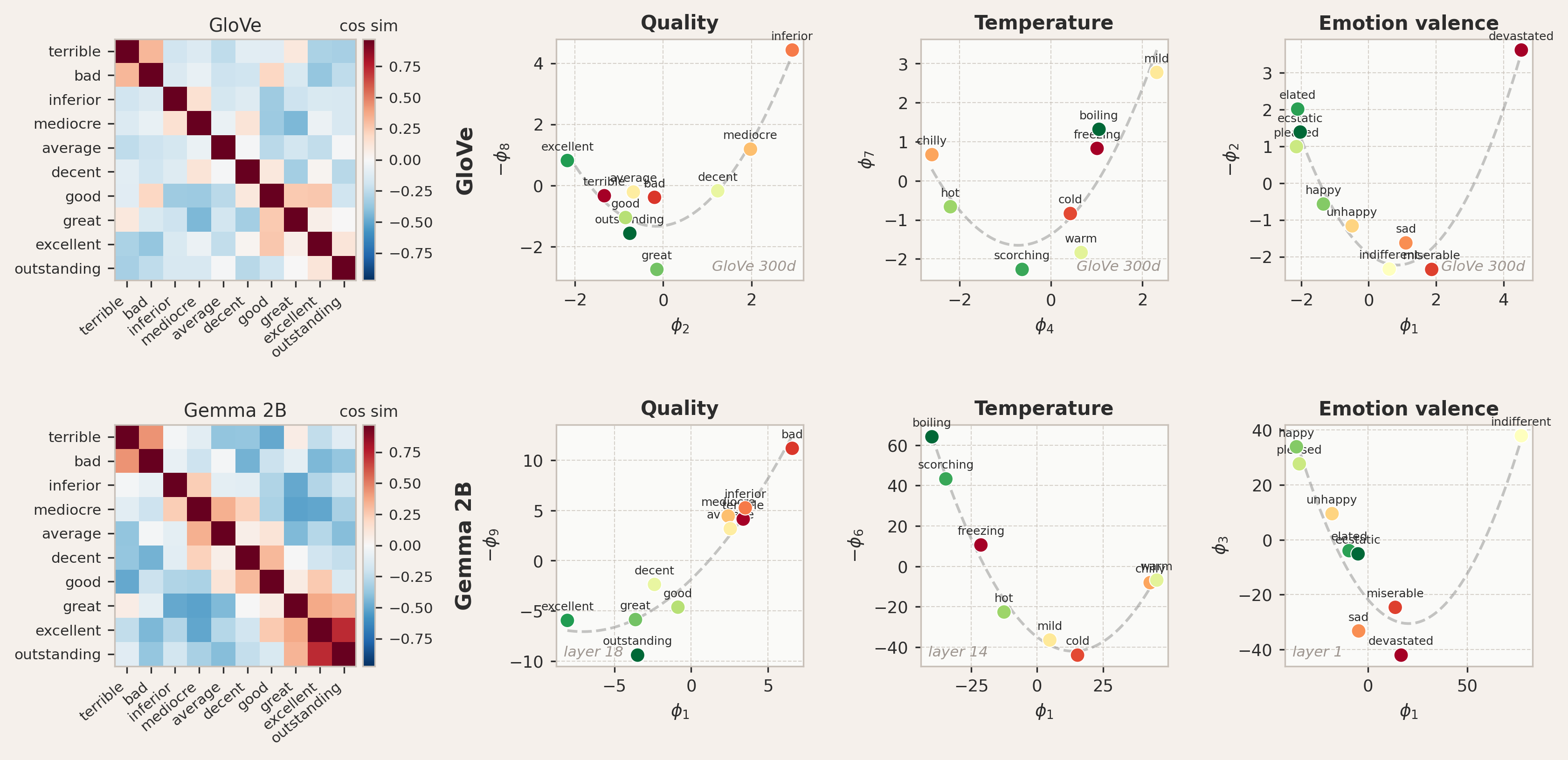
Testing the Neumann prediction for quality, temperature, and emotion valence. The embeddings lie on the theoretically predicted parabola, despite some perturbations in ordering. In GloVe, the parabola appears in different PC pairs: quality (
Interestingly, the ordering along the parabola does not always match the ranking we would intuitively assign. The parabolic geometry is a consequence of the boundary condition alone and holds for any set of tokens governed by Neumann conditions, regardless of their spacing. The ordering, by contrast, depends on the positions
Logarithmic scales
I also tested concepts that vary over many orders of magnitude, such as storage capacity (byte to exabyte), temporal duration (second to millennium), and monetary value (cent to trillion). In contrast to the ordinal scales above, the assumption of uniform spacing breaks down here. The semantic distance between a kilobyte and a megabyte is not the same as between a megabyte and a megabyte-plus-one-kilobyte. What matters is the ratio between adjacent levels, not their difference, for which the meaning-carrying structure is logarithmic.
This changes the boundary conditions. Logarithmic scales are asymmetric by nature. The lower end is anchored at a definite smallest value: the scale of storage starts at a byte, monetary value at a cent, and so on. These are not fundamental limits, but they mark the point where each concept begins. The upper end, by contrast, is open-ended; there is no natural maximum to storage or money, so the scale is free there. This asymmetry calls for mixed boundary conditions: Dirichlet at the lower end with
where
which maps the range of physical values onto the interval

For logarithmic scales, mixed boundary conditions apply: Dirichlet (pinned) at the lower end and Neumann (free) at the upper end. Atoms spaced uniformly in log-space (right) produce qualitatively different mode shapes than linear spacing (left). Theory predicts sinusoidal modes when plotted against the normalized log-position
The analysis also differs slightly from the ordinal case in how the modes are extracted from the data. For ordinal scales, theory predicts the parabola to live in a specific two-dimensional plane in PC space, so the first two principal components directly reveal the geometry. For logarithmic scales, there is no reason the relevant mode should align with the first principal component. To test the prediction, we search over the top principal components to find the one whose values most closely follow a quarter-sine profile
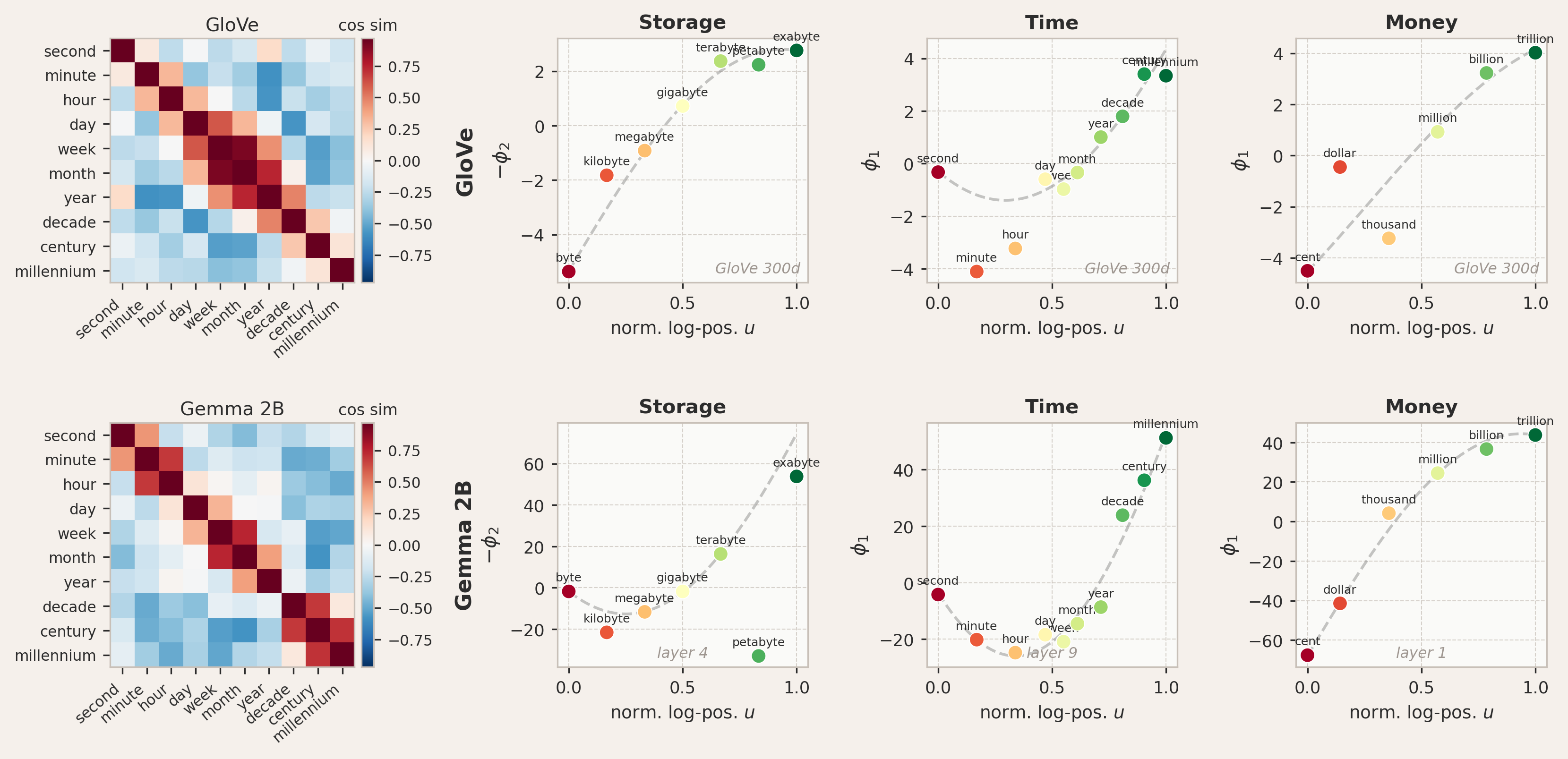
Testing the mixed Dirichlet-Neumann prediction for storage, time, and monetary scales. Shown is the best-fitting principal component projected against the normalized log-position
Testing these three concept sets in both GloVe and Gemma 2B, we find confirmation of the predicted mode shapes. In GloVe, storage and money show good agreement with the first mode, with the tokens tracing the quarter-sine arc when plotted against their log-positions. Time conforms better to the second mode, displaying a half-sine shape. Gemma 2B also shows good agreement with the theoretically predicted shapes, particularly for time and money. Storage in Gemma is the weakest case: the best-matching principal component captures essentially no variance, meaning the sinusoidal pattern, while present, lives in a direction that is geometrically irrelevant to the overall embedding structure. This may indicate that the logarithmic storage hierarchy is not a salient feature of Gemma's representations at the tested layer, or that the signal is distributed too thinly across many components to be recoverable from a single PC.
Also, the fact that different concepts and models favor different modes (e.g., mode 1 for money vs. mode 2 for time) is not entirely unexpected: the theory predicts a family of modes, and which one best matches a given concept depends on the eigenvalue spectrum of the co-occurrence kernel. The eigenvalues determine how much variance each mode captures, and their relative magnitudes are shaped by the training data, the tokenization, and the model architecture.
2D concepts - Russell circumplex
The previous experiments all dealt with one-dimensional semantic scales. But many concepts are inherently two-dimensional. A classic example is the Russell circumplex model of affect, which organizes emotions along two independent axes: valence (unpleasant to pleasant) and arousal (calm to excited). If the phonon framework extends to two dimensions, the 2D Neumann modes
Interestingly, a very recent study by Anthropic's interpretability team provides independent evidence that this structure is real. They extracted 171 emotion vectors from Claude Sonnet 4.5 and found that the top two principal components of the emotion vector space align with valence (

The 2D Neumann boundary condition applies to concepts varying along two independent semantic axes. Mode (1,0) captures variation along one axis only, while mode (1,1) encodes the interaction between both dimensions. This is tested using data from the NRC VAD Lexicon (Mohammad, 2018), which provides crowdsourced human ratings of valence and arousal for each emotion word.
To test this, I selected 69 emotion words spanning all four quadrants of the circumplex, from high-arousal negative (terrified, enraged) to low-arousal positive (serene, tranquil). Each word is assigned a coordinate
Experimental details
Word set and coordinates: I selected 69 emotion words spanning all four quadrants of Russell's circumplex model of affect, from high-arousal negative (terrified, enraged) to low-arousal positive (serene, tranquil). Each word is assigned valence and arousal coordinates from the NRC VAD Lexicon (Mohammad, 2018), a database of human ratings for over 20,000 English words. The ratings were collected via crowdsourcing using Best-Worst Scaling, where annotators were shown sets of four words and asked to identify the one with the highest and lowest intensity along a given dimension.
Embedding extraction: I used Gemma 2 27B in bfloat16 and extracted hidden states using last-token pooling as before. The prompt template was The person is feeling {word} . A layer sweep over layers 1 through
PCA and mode fitting: The
So we ask which mixture of PCs best matches a given mode. The fitted value

Testing the 2D Neumann prediction on 69 emotion words from Russell's circumplex model, using Gemma 2 27B at layer 28. Left: mode
The results are shown for two modes. The left panel shows mode
Outlook
These are early results, but very encouraging ones. Karkada et al. (2026) showed that the twelve months of the year are embedded as a near-perfect circle in the activations of Gemma 2B, a geometry that follows from periodic boundary conditions applied to a cyclic concept. The mathematics they used is just an excerpt from the broader frameworks developed in solid-state physics to study crystal vibrations. I tested whether this connection extends beyond a single case by applying different boundary conditions to different semantic concepts, and found confirmation for periodic, Neumann, mixed, and 2D Neumann geometries. Much more work is needed to establish how robust and general these patterns are, but the basic premise, that the geometry of word representations can be derived from physical principles applied to the semantic structure of a concept, appears to hold.
I find it noteworthy that just around the time of this writing, a paper appeared on the arXiv (accepted at ICLR 2026) titled "The Lattice Representation Hypothesis of Large Language Models". The author shows that LLM embeddings encode not just individual concepts but the algebraic structure of a concept lattice, with operations like meet and join recoverable directly from the geometry. If this lattice structure is real, the phonon modes I proposed could just be the vibrational modes of exactly that lattice, with the boundary conditions set by the local topology of the concept graph. The lattice would provide the structure, and the phonon framework the dynamics. This is speculative, of course.
I am currently exploring how the phonon picture can be extended to additional boundary condition types, to higher-dimensional semantic structures, and how different modes might interfere with one another and what such interference would actually mean. The goal is to find a theoretically grounded description of how models represent meaning internally. The recent finding by Anthropic's interpretability team that emotion representations in Claude causally drive alignment-relevant behavior, and that these representations organize along the same valence-arousal geometry that the 2D phonon modes predict, suggests that this line of research may have practical consequences beyond interpretability. My hope is that a principled understanding of how concepts like morality or harm are geometrically encoded could offer a path toward understanding and enforcing alignment.

Acknowledgments
Thank you to Dhruva Karkada, Lysander Mawby, and Marvin Koss for feedback :)
Discuss