This is a first in a pair of posts I’m hoping to write about Singular Learning Theory (SLT) and singularities as a model of data degeneracy. If I get to it, the second post is going to be more general-audience; this one is more technical.

Introduction

To me, SLT is an important source of toy models which point at an interesting class of new statistical phenomena in learning. It is also a valuable correction to an older and (at this point) largely-defunct story of learning being fully controlled by Hessian eigenvalues and “nonsingular basins”. Practitioners of SLT have been instrumental for developing and refining the practice of Bayesian sampling (used by physicists in papers like this one) to empirical models. And the theory’s founder Sumio Watanabe is a once-in-a-generation genius who saw and mathematically justified crucial statistical and information-theoretic concepts in ML long before they appeared in “mainstream” theory.

However there is a frequently repeated statement in SLT papers – one that doesn’t affect empirical results – which I think is wrong in a load-bearing way. This is the statement that models that appear in machine learning are singular in the infinite-data limit, and that a measurement associated with this singularity, called the RLCT, controls generalization and free energy in cases of interest.

This isn’t a fixable detail, but rather an unavoidable structural issue I’ll spell out below. I think it’s unfortunate that an elegant and useful theory is linked with an incorrect statement, and it causes potential for future disappointment and for research stuck in a less-useful direction. Many theory and empirics results associated with SLT are important and, I think, interpretability-relevant, independently of the question of whether singularity “explains degeneracy” in practice. As I’ll explain below, I think that singular models correctly occupy the same role as symmetries in condensed-matter physics. Many key phenomena, in particular symmetry-breaking phase transitions, were originally discovered in more idealized models with symmetry, but the resulting physical phenomenology extends to a huge class of phase transitions of models with no symmetry involved.

I’ve explained to several people the key arguments for why the singularity story is flawed. Several (most recently Yevgeny Liokumovich, to whom I’m indebted for really good discussions) liked the key example and asked me to write this up – so I will do so in this post. In this post I’ll focus on the more subtle second part of the statement (the first part – whether ML models are singular at all in the infinite-data limit – is the subject of the future companion post). I’ll show that the true degeneracy, correctly measured by the lambda-hat parameter,^[1] is in fact much stronger in realistic learning contexts, and hence generalization behaves much better than a purely singularity-based prediction would imply.

The key insight of this post is contained in the Hermite mode graph below. It shows that even upon biasing the odds in favor of the SLT theoretical model: looking at a clean, singular model where the SLT limit is understood, its regime of applicability only sets in at astronomically large (roughly exponential in model size) data. At any realistic data scale, the load-bearing structures that control degeneracy cannot be (at least exclusively) associated with singularities, and require a distinct thermodynamic notion of “effective theory” which is not purely geometric.

What doesn’t need fixing

First, let me say some things that I believe to be true quite generally, and do not need fixing in the SLT story:

• Model generalization in the Bayesian regime is controlled by measurements of free energy of a low-loss basin (i.e. the region of the loss landscape where the loss is between two values and where is the best possible loss in the basin).
• Understanding this low-loss basin for different , and understanding its geometric, physical and information-theoretic properties is valuable for interpretability. In particular there is much evidence that in practice, learning-relevant phenomena in Bayesian settings occur also in other kinds of learning (such as SGD).
• For models that generalize well, this basin will tend to be larger. (There is a version of this that is a theorem.)
• The size of this basin at a given loss sensitivity parameter can be measured via the “lambda-hat estimator”, which is often (informally) called the (estimated) “learning coefficient” in SLT papers^[2] (and converges to the true lambda-hat value in a suitable limit).

What’s wrong

What is false here is that the measured value lambda-hat captures information that is primarily the geometry of a singularity in any cases of interest. In particular the nomenclature “learning coefficient” (which is a geometric invariant of a singularity) is incorrect in almost all settings.

There are two settings where identifying lambda-hat with geometric information makes sense:

1. A version of it is true and useful for highly-symmetric tasks on linear models and for shallow quadratic models (for example in this paper).
2. A version of this is true for models of very low dimension (order of magnitude of perhaps 20 parameters), as seen in e.g. this paper.

However outside of these two cases singularities are not the right measurement to understand generalization, at least when taken by themselves. The key issue (that I hope to expand a bit in the companion post) is that the phenomenon of a loss function being singular is unstable. This is similar to how a general continuous function on an interval is not a polynomial (though it can be arbitrarily well approximated by a polynomial spline). Thus asking “what is the singularity controlling generalization of a task” can be similar to asking “what is the polynomial degree of the function “. There may be invariants similar to polynomial degree that are interesting, but the notion of degree by itself as a nice algebraic invariant breaks down.

I think that to see how the singularity story breaks down it’s best to look at a setting where the theory actually works perfectly in the limit, but exceptions (1) and (2) above don’t hold. This means that we should look at a model:

1. With non-polynomial activations and
2. With (mildly) high parameter dimension.

We’ll furthermore take a setting with a nontrivial and well-understood singularity.

The best example here is to consider a 2-layer model learning the zero function

Here the story I’ll tell depends a lot on the activation function (though the general “generalization behavior” is broadly activation-independent at more permissive values of ). Let’s choose the activation function (this is associated to a cleaner energy function as we’ll see). To make life easier, let’s write down a model without biases^[3]:

Here are h-dimensional vectors ( for “hidden dimension”).

In particular the parameter dimension in this case is To have “moderately high parameter dimension” let’s take h = 128, so .

The theory

So far we haven’t talked about data. When we have a learning problem, we should have a data distribution on inputs . In this case the inputs are in a 1-dimensional space and a natural distribution is the normal (Gaussian) distribution of variance one:

In particular when we are talking about loss singularities, we care about the infinite data loss. In other words loss averaged over all drawn from this distribution. It is nevertheless conventional to also include a parameter in SLT analysis, which is the number of training samples. Recall that I used a “basin height” value to define the basin volume (if we directly set , the volume is zero and the entropy is ). In physics, this is called the temperature^[4].

Infinite data, and the parameters and .

In SLT work, the value is replaced by a multiple of .^[5] Importantly, Watanabe proves that in order to get accurate information about the loss minima within accuracy, one needs on the order of datapoints (up to some logarithmic factors that we can ignore – for mathematicians, our asymptotic notation should be read as “tilde-notation” here). While this is proven at an asymptotic scale, it is borne out at realistic scale in toy models (more generally one direction of the associated inequality can be established in much more generality).

This means that typically for a deep network, measuring the infinite-data loss of a given neural net to accuracy requires on the order of data points. It turns out that for one-layer networks, one can often circumvent actually taking data averages and compute the infinite-data loss directly, or at least to exponential accuracy. Indeed, the infinite-data loss is an integral, and integrals can often be rewritten via (something like) a Taylor series, with exponential rate of convergence. In the 2-layer case, a nice formula to use is the Gauss-Hermite quadrature formula.

The SLT prediction

Before going on, let’s write down the SLT prediction, which is clean in this case. SLT theory predicts that in the true limit, the value of lambda-hat will stabilize to a known value associated to the singularity, called the RLCT. For a generic loss function, the expectation here is that the RLCT is (this is for example true for the problem of learning a single Hermite mode, such as .^[6]

Here we are in a highly symmetric case, and the target has a true degeneracy. Moreover it is singular at the point . The singularity can be well understood here (this is an important SLT result), and we have:

(To see this: note that if we take , the output is always the zero function, no matter what we choose for . This leaves us a degeneracy of dimension , which implies a bound of . There are other 64-dimensional degenerate subspaces, for example ; but we can check by analyzing the singularity that the added degeneracy produced is not strong enough to reduce the RLCT).

This implies that in the limit , the asymptotic lambda-hat measurement must return 64. The key wrinkle shows up when we look at what “the limit” actually entails.

Hermite modes and excitations

For finite , we can heuristically estimate the lambda-hat value, and the number of degrees of freedom, in a different way. The resulting value for measures the effective degeneracy at a finite dataset, and is the relevant quantity for generalization at the corresponding dataset size.

Recall that we’re learning the zero function . This means that in the space of functions, the loss of a given function (maybe given by a weight parameter ) is where is the Gaussian pdf “data distribution” function. We can rewrite this integral as

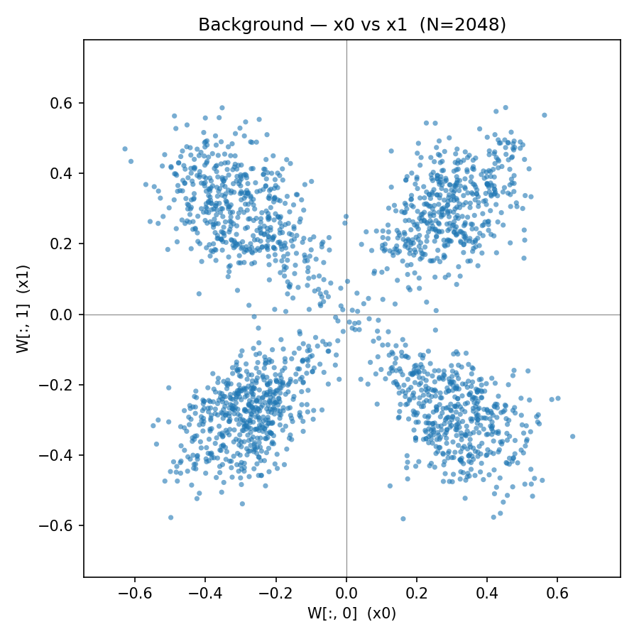
Here the numbers are the coefficients of in an elegant orthonormal basis called the basis of Hermite polynomials. Now for neural nets with an analytic activation function (such as tanh), we can show that this series not only converges but it converges very quickly. In particular, the following is a logarithmic plot of the coefficients for a random neural net of width , where the embedding weights are uniformly chosen between -1 and 1:

Note that I’m using the Gauss-Hermite quadrature formula here to compute the infinite-data function to accuracies of this order. In order to get comparable accuracy with random sampling I’d have to use on the order of samples, more than the training corpora for the biggest existing models. The scaling law on the square Hermite coefficients behaves asymptotically like , and we can even theoretically predict the slope^[7].

We can think of this situation as a physical system with many different excitation modes indexed by the integer k. Higher modes are “heavier”, or harder to excite. They become relevant only as we require more precision (or “degree of resolution”) of our system – in physics lingo they are “UV modes”.

An upshot for the lambda-hat calculation is that so long as our value n (corresponding to the number of samples or ) is significantly less than , the kth mode doesn’t matter: we can completely ignore loss coming from that mode. In particular, so long as our number of samples is less than or so, the space explored by the model has effectively less than 100 degrees of freedom. By a simple argument we can then deduce that any lambda-hat value measured at datapoints is less than (the measure roughly counts the number of “effective degrees of freedom”). This is important enough to write out explicitly:

Note that (a more careful version of) this inequality is easy to prove rigorously by making formal the Hermite mode decay arguments above.

This inequality shows that we can’t even begin to saturate the “true singularity” RLCT = 64 before exponentially high numbers of data.

This means that we have demonstrated the following observation:

In order to see the true RLCT in a simple 256-parameter singular model, we need a data sample of size

In practice, the free energy (and the associated lambda-hat measurement) is much lower at any “realistic” data scale. This is actually good, and what we expect: it’s saying that “return roughly to 0” is actually very easy to learn, and requires very little data in practice.

Addendum: the actual lambda-hat scaling (Ansatz and experiment)

To prove that the effective degeneracy value undershoots the RLCT, we used an inequality between and which I believe is straightforward to make rigorous. This leads to a natural Ansatz that this is an asymptotic equality up to a suitable factor, and is a quadratic function of . The Ansatz here comes from the Hermite mode scaling: any value of n sees at most Hermite modes as relevant degrees of freedom. If we were to assume these have no relations between them, the lambda-hat scaling would be exactly .

From this we get a prediction that the free energy in this setting is cubic in log-n:

This contrasts with the SLT limit where the free energy is linear in

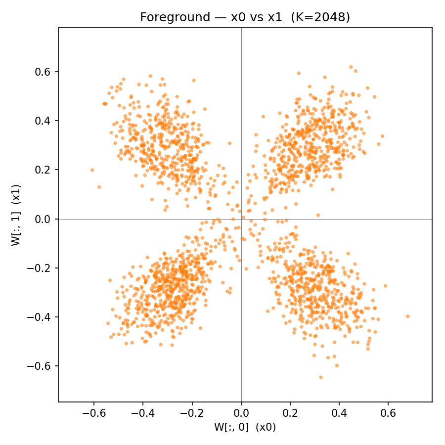
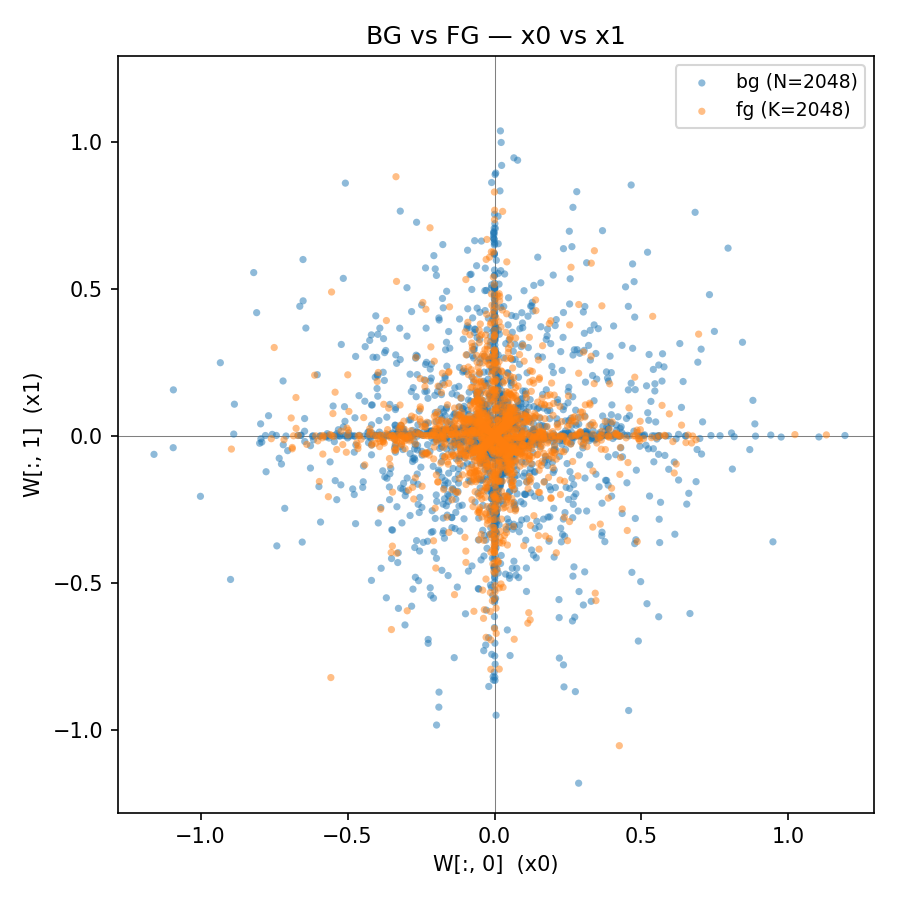
I ran a sampling experiment to confirm this, and the result agrees with the Ansatz. In the graph the parameter (beta) is what I was calling n here.^[8]

It’s worth reiterating that this quadratic behavior is very much an effective phenomenon as we change the scale of interest. In the true singular limit (very large n), this roughly quadratic growth should plateau out at .

Measuring lambda-hat depends on sampling at low temperatures, a notoriously finicky process, so it’s plausible that the measurement in this experiment is flawed. Extrapolating this graph, we would expect the RLCT to plateau to the true value at roughly , or when roughly Hermite modes become relevant.

The effective theory

In the previous sections we have been contrasting a purely geometric SLT prediction with a physical effective theory which posits a sea of coupled excitation modes that gradually become relevant at larger and larger n. Note that the improved theory does not predict that the free energy is captured by the Hessian eigenvalues (thus reducing it to the defunct “classical learning theory” that assumes all basins are quadratic). Indeed, all Hessian directions in our example are exactly zero, and any meaningful theory must see the singularities. The reality here instead is that the singularities are not the whole story. In order to understand the way that a network of any realistic size learns, we need to understand a physical volume. This volume can have “hard” geometry at the limit (singularities). But it can also have “soft” geometry, where for finite values of the valley has real finite “thickness” parameters that scale differently in different regimes. In some cases these can be viewed as generalized and nonlinear “widths” of the basin’s free directions. Since the number of free directions is huge and thicknesses combine multiplicatively, these can (and in our example do) easily dominate the limiting singular structure (if it exists) at any “sub-astronomical” data size. These numerical widths can come from Hessian eigenvalues, or they can happen in a Hessian-flat region and combine with singularities as in the example above. More generally the free energy measurements can see complicated thermodynamic structure nonlinearly coupling numerical size parameters associated to many degrees of freedom.

Physics has a set of tools for understanding such high-dimensional structures that interacts richly with the energy scale, and these physics approaches have been applied in an ML context. The best tools we have tend to come from multi-particle thermodynamical systems, where numerical and geometric degrees of freedom of microscopic particles combine nontrivially to give an effective energy landscape on macroscopic parameters.

One setting where this is done cleanly is the body of knowledge known as “NN field theory”. This theory exists in a large-width limit and is, like SLT, incomplete. But it has the advantage of giving the correct effective theory for models with simple targets which have “reasonably large” size, giving a kind of complement to SLT.

This theory is undergoing active development in a manner that resembles the SLT update with respect to the old “Hessian basin” story. In this case an old story of Gaussian processes is being extended to a much more expressive theory, by expanding around a nontrivial/ strongly-coupled vacuum – aka a mean field theory. In cases where they apply, these theories tend to come pre-equipped with a hierarchy of effective theories that for example extend the Hermite excitation story above.

A theory that combines mean field and singularities is much needed. In fact the existing statistical field theory literature already can account for simple cubic and quartic singularities, called “Airy” and “Pearcey” corrections, respectively, but we currently lack a more unified low-temperature picture that can track general singularities. There’s an interesting potential precedent here: when physicists observed tensions between large symmetry groups and field theory, the resulting notion of gauge theory unified the two fields and generated a new family of insights that transformed modern physics. Building a corresponding theory for singularities – a theory that combines singular phenomena with high-dimensional field theoretic phenomena in neural nets – strikes me as an unusually promising direction for a version of SLT that is empirically faithful while retaining interesting geometric structures (though it should be noted that singularities without additional structure are pretty significantly different from symmetries in a physics setting, and the analogy is not guaranteed not hold up).

Is this example special?

The example is chosen to be clean, but the conclusion doesn’t depend on its cleanness; if anything, the gap between the singular prediction and reality widens in messier settings. Settings where a clean physics story is known are very rare, but similar (and indeed nicer, though slightly less “natural-seeming”) examples exist. The choice of activation function and data distribution generalizes completely: so long as the activation is analytic, it’s relevant in terms of the details of exponential growth rather than its presence. In particular a very nice context to use (that I considered building this post around) is a two-dimensional input distribution restricted to a circle , where the different excitation modes correspond to group representations^[9] and the exponential growth of energies at different degrees is cleaner. A similar (though more complicated) story exists for the cube in d-dimensional space.

But moving away from this kind of clean setting cuts in a particular direction: it makes both sides of the picture worse, not just one. Higher-dimensional or less regular data or non-analytic activations give messier spectra^[10] (or no clean spectrum at all), and the same features also weaken the singular structure that SLT needs. Genuine singularities for NNs at infinite data are a feature of analytic, low-dimensional models; making the model less clean tends to wash them out. Depth introduces a separate problem. Denoising effects (learned by realistic models) can turn high-loss solutions of a shallow network that are far from a potential singularity into very low-loss solutions that are indistinguishable from singular minima at any sub-astronomical n, even though they are not singular in the SLT sense.

Ultimately I’m sympathetic to SLT phenomena “contributing in a relevant way” to models (more in the next section); but my honest view is that as we move away from this clean example, the possibility of singularity fully explaining degeneracy at realistic scales becomes more and more remote.

The upshot

At the end of the day, my personal view is that loss landscape singularities do matter for realistic models. But the way they matter happens at specific, relatively coarse, values of the cutoff , and in low-dimensional reductions – like the low-dimensional Fourier modes of modular addition, or otherwise localized components of a larger and messier model. They should only be visible once the dominant – but likely less interesting – bulk effects (like the above spectra) have been taken into account. To me this picture is very similar to the story of symmetry in statistical physics. Here symmetry groups typically produce neat and mathematical corrections – factors of 2 and the like – to messier statistical effects special to large systems. Though sub-dominant, the structures associated with symmetry are often instrumental for crystallizing out new structures and phenomena. I also buy Watanabe’s reasoning that singularities, more than symmetry, cause interesting degeneracy and generalization behavior in the statistical physics of learning models. This makes it likely that singularities are a “fundamental idealization” in learning similar to how symmetries are a “fundamental idealization” in physics.

Nevertheless this is speculation. The solid corrective to take home is that degeneracy in realistic models should not be too readily identified with singularities. The SLT notions of “effective degeneracy” and free energy remain valuable whether or not the degeneracy is produced by singular structure, and the lambda-hat estimators that measure these values (always at a finite or effective scale!) remain well-grounded. The effective story is crucial for learning, but is not necessarily geometric. In the cases where these are best understood, and in fact where singularities most cleanly appear, the actual “hard” singular structure is only visible at data sizes larger than the size of the visible universe.

As usual, reality is more complicated than a simple story. And as usual, the simple stories point at real phenomena that are incredibly important for reality.

1. ^{^}

   The terminology “lambda-hat” for an important and easy-to-measure physical quantity is unfortunate. It seems that physics lacks a more canonical name for it. I’ll stick with lambda-hat for this post.

2. ^{^}

   Mathematically, the lambda-hat estimator converges to more or less the derivative of the free energy, i.e. roughly the “entropy”, or log volume, of the basin with respect to epsilon: this follows a standard pattern in physics where derivatives of the free energy tend to be easier to compute than the energy itself. The full free energy can be computed by taking a numerical integral of this value (appropriately scaled) over different epsilon. In practice, if we are interested in a ballpark measurement of the free energy, just taking lambda-hat at a single cutoff of interest is sufficient, and tends to be associated with generalization in the way you want.

3. ^{^}

   This doesn’t matter for the asymptotics here.

4. ^{^}

   In both physics and SLT, the basin “walls” are not hard step functions at loss = but rather soft “logistic” walls – this doesn’t change the phenomenology in practice.

5. ^{^}

   The law often has a log factor in SLT papers, so or similar. As it’s a small multiplicative factor compared to , it’s often ignored. When working straightaway with infinite data as we will be doing, the important variable is the “temperature” and setting is a notational choice.

6. ^{^}

   Note that in our model readout weights are regularized, which leads to the same asymptotic as having readout weights be bounded, so we can’t cheat by for example writing .

7. ^{^}

   We can in fact read off the exact asymptotic multiple here from the Hermite coefficients of the function. The value here (doubled since we’re looking at the square coordinates) is the minimal distance of a pole of the analytic continuation of the hyperbolic tanh function from the real line: tanh is singular at , since .

8. ^{^}

   Recall that in our loss valley discussion, the valley’s “height” is a temperature parameter, and is an inverse temperature parameter, often denoted beta.

9. ^{^}

   I think the circle in particular is a mathematically very nice example. The spectrum there is, in particular, exponential without a square root.

10. ^{^}

    In particular non-smooth activations like relus have less extreme spectra at infinite data.

Discuss

This is the first post in a planned series about mean field theory by Dmitry and Lauren (this post was generated by Dmitry with lots of input from Lauren, and was split into two parts, the second of which is written jointly). These posts are a combination of an explainer and some original research/ experiments.

The goal of these posts is to explain an approach to understanding and interpreting model internals which we informally denote “mean field theory” or MFT. In the literature, the closest matching term is “adaptive mean field theory”. We will use the term loosely to denote a rich emerging literature that applies many-body thermodynamic methods to neural net interpretability. It includes work on both Bayesian learning and dynamics (SGD), and work in wider “NNFT” (neural net field theory) contexts. Dmitry’s recent post on learning sparse denoising also heuristically fits into this picture (or more precisely, a small extension of it).

Our team at Principles of Intelligence (formerly PIBBSS) believes that this point of view on interpretability remains highly neglected, and should be better understood and these ideas should be used much more in interpretability thinking and tools.

We hope to formulate this theory in a more user-friendly that can be absorbed and used by interpretability researchers. This particular post is closely related to the paper “Mitigating the Curse of Detail: Scaling Arguments for Feature Learning and Sample Complexity“. The experiments are new.

What do we mean by mean field theory

Mean field theory is a vague term with many meanings, but for the first few posts at least we will focus on adaptive mean field theory (see for example this paper, written with a physicist audience in mind). It is a theory of infinite-width systems that is different from the more classical (and, as I’ll explain below, less expressive) neural tangent kernel formalism and related Gaussian Process contexts. Ultimately it is a theory of neurons (which are treated somewhat like particles in a gas). While every single neuron in the theory is a relatively simple object, the neurons in a mean field picture allow for an emergent large-scale behavior (sometimes identified “features”) that permits us to see complex interactions and circuits in what is a priori a “single-neuron theory”. These cryptic phrases will hopefully be better understood as this post (and more generally as this series) progresses.

Why MFT

We ultimately want to understand the internals of neural nets to a degree that can robustly (and ideally, in some sense “safely”) interpret why a neural net makes a particular decision. So one might say that this implies that we should only care about theories that apply directly to real models. Finite width, large depth, etc. While this is fair, any interpretation must ultimately rely on some idealization. When we say “we have interpreted this mechanism”, we mean that there is some platonic gadget or idealized model that has a mechanism “that we understand”, and the real model’s behavior is explained well by this platonic idealization. Thus making progress on interpretability requires accumulating an encyclopedia (or recipe book) of idealizations and simplified models. The famous SAE methodology is based on trying to fit real neural nets into an idealization inherited from compressed sensing (a field of applied math). As we will explain below, if we never had Neel Nanda’s interpretation of the modular addition algorithm, we would get it “for free” by applying a mean field analysis to the related infinite-width model. As it were, the two use the same Platonic idealization^[1]. Thus at least one view on the use of theory is to see it as a source of useful models that can be then applied to more realistic settings (with suitable modification, and, at least until a “standard model” theory of interpretability exists, necessarily incompletely). Useful theories should be simple enough to analyse mathematically (maybe with some simplifications, assumptions, etc.) and rich enough to illuminate new structure. We think that mean field theory (and its relatives) is well-positioned to take such a role.

Brief FAQ section

“Frequently asked questions about MFT” is a big topic that can be its own post. But before diving into a more technical introduction, we should address a few standard questions which keep cropping up, especially about comparisons between MFT and other better-known infinite-width limits.

1. Doesn’t infinite width mean that we’re in the NTK (or more generally a Gaussian process) regime? The first analyses of neural nets at infinite width have been in the so-called NTK regime, where in particular the model “freezes” to its prior/ initialization at all but the last layer (which is performing linear regression). This is a remarkably deep picture that is for example sufficient to learn mnist. But approaches in this family exhibit extremely different behaviors from realistic nets (in particular the freezing of early neurons) and they are generalize much worse on problems that cannot be solved by some combination of clustering and linear regression (of which MNIST is an example). For example these methods learn only memorizing circuits in modular addition (at least in known regimes) and, worse, they are known to require exponential training data and complexity for learning algorithms that are well-known to be learnable by SGD (see for example the leap complexity paper) – this means that these techniques are fundamentally incompatible with these settings (more generally so-called “compositional” models – ones that have multiple serial steps which models tend to need depth for – have similar failures in this regime). This can be partially improved by including so-called “correction terms”, but these only work when the Gaussian process has good performance by itself, and fail to ameliorate for the exponential complexity issues. Note that the Gaussian process picture is useful as a heuristic baseline. In particular it makes some predictions on scaling exponents that have some experimental agreement (and is related to the muP formalism).

   It turns out that the lack of expressivity of the Gaussian limit is due not to its having infinite width to a certain choice of how to take the infinite limit (and in particular how to scale weight regularization terms in the loss). Different limits and scalings give significantly more expressive behaviors as we shall see, and we use MFT as a catch-all term for these. (These different limits are also harder in general, at least in terms of exact mathematical analysis: the Gaussian process limit somewhat compensates for its lack of expressivity by having much easier math.)

2. Isn’t mean field theory only a Bayesian learning theory and doesn’t that make it unrealistic? In physics contexts (like MFT, Gaussian Process learning, etc.) Bayesian learning is often theoretically easier to deal with, and we’ll explain Bayesian learning predictions here (validated by tempering experiments). However a version of mean field for SGD learning exists and is called “Dynamical Mean Field Theory” (DMFT) (it extends the NTK in Gaussian process contexts). Probably more relevantly, Bayesian learning experiments frequently find similar structures to gradient-based methods (and are often easier to analyse). This is particularly well demonstrated in empirical results by the Timaeus group.
3. Is mean field theory a theory of shallow models? Most existing papers on mean field theory work in the context of 2-layer neural nets (i.e. 2 linear layers, one nonlinear layer). However there is a fully general, and experimentally robust extension of the theory to a larger number of layers (see for example this lecture series), and we will look at such models here. In fact mean field theory can model mechanisms of arbitrary depth – but it works best for shallower models (or for shallow mechanisms in deep models), and would likely be less useful for modeling strongly depth-dependent phenomena.
4. What is a success of mean field theory I should know about? Glad you asked! Most people know about the Modular Addition task, which was first explained mechanistically by Neel Nanda et al.’s grokking paper. The interpretation is heuristic: it shows that the model exhibits signatures of using a nice and unexpected trigonometric trick. It also interpolates between generalization and memorization in a sudden shift reminiscent of a phase transition. A more ambitious task (that was considered too hard to tackle in the interpretability community) would be to understand exactly what the model learns on a neuron-by-neuron basis in any setting that exhibits generalization/ grokking. Since models have inherent randomness (from initialization, and sometimes from SGD), the task is inherently a statistical one: explain the probability distribution on weights of learned models (at least to a suitable level of precision), and was generally believed to be quite hard. Thus it comes as a surprise to practitioners of interpretability that in fact there is a context where this is done.

   In the paper “Grokking as a First-order Phase Transition in Two Layer Networks“, Rubin, Seroussi and Ringel constructed a complete explanation (experimentally verified to extremely high precision) for the modular addition network in the Bayesian learning setting (there are some other differences from Neel Nanda’s approach, most notably the choice of loss function, but variants of the approach extend to these as well). The distribution is first understood at infinite width, then shown to apply at realistic (but large) width in the appropriate regime. When applying the adaptive mean field theory approach to this task, Fourier modes and the trigonometric mechanism fall out as a natural output of the theory – moreover they are fully explained on a statistical distribution level (i.e. we have a complete model “exactly what each neuron does” to an appropriate degree of precision, understood in a statistical physics sense). Of particular interest, the model explains a grokking-like phase transition between memorization (equivalently, a Gaussian process-like behaviour) and generalization (inherently mean field) and predicts the data fraction at which it happens (this is a Bayesian learning analog of predicting the distribution of when grokking happens in SGD-trained neural nets). The phenomenon is a genuine phase transition in the thermodynamic sense.

5. Are real models in the mean field regime or the Gaussian process regime, or something else? This is an interesting question, whose answer is “this question doesn’t make sense”. The distinction between regimes applies to infinite width nets, i.e. to a totally non-standard setting. One can prove rigorous results with the gist that if the width is (sufficiently enormous with some giant bound) compared to the training data, the model is guaranteed to learn in one of these two regimes. However, no real models are that enormous. Instead, some phenomena and some mechanisms can be seen (experimentally or theoretically) to extend from infinite nets to nets of finite width. Sometimes these look more like mean field phenomena, sometimes they look like Gaussian process phenomena. For example in some sense MNIST is “GP-like” (GP stands for Gaussian process). Circuits in modular addition are, as it turns out, entirely explained by the MFT limit as we’ve explained above.

Introduction to the theory

The background (and the foreground)

In physics, one often looks at systems with a large, stable background. A planet vs. a sun, an electron vs. a proton, a weakly interacting observer vs. a large system being observed. In these settings the “background” is the large system and the “foreground” or “test system” is the small system being studied. In these cases the background system may be fixed, or it may be undergoing some motion (like the sun moving around the galaxy’s center), but the important idealization is that it does not react to the observer/ test system. In fact, the earth is applying a gravitational pull to the sun (and famously in quantum mechanics, observations always impact a system at a quantum level). But these “reverse” effects are small, so to a good approximation we can treat the sun as doing its own “stable” thing while earth is undergoing physics that depend strongly on the sun.

Self-consistency

While typically the large “background” is a cleanly separate system from the small test system of the observer, it is sometimes extremely useful to treat the test system as a tiny piece of the background. So: the large background system may be a cup of water and the small test system may be a tiny bit of water at some location. Here while technically the full cup includes the tiny “test” bit, the large-scale behaviors (waves etc.) in the water don’t really care to relevant precision if the test bit is changed or removed (at least if it’s tiny enough). But the tiny bit of water definitely cares about the large-scale behaviors (waves, vortices or flows, etc.), to the extent that bits of water care about things.

Similarly (and in a closely related way), “the economy” is a giant system that includes your neighborhood bakery. The bakery can be viewed as a small “test system”: it is affected by the economy. If property prices go up or the economy tanks, it might close. But the economy is not (at least to leading order) affected by this bakery. It is perhaps affected by the union of all bakeries in the world, but if this particular bakery closes due to some random phenomenon (e.g. the lead baker retires), this won’t massively impact the economy.

This point of view is remarkably useful, because it introduces a notion of “self-consistency”.

Self-consistency when applied in this context comes from the following pair of intuitions:

1. the behavior of each small component is (statistically) determined by the background
2. the behavior of the background is the sum of its small components.

If both of these assumptions are true, then these two observations (when turned into equations) are usually enough to fully pin down the system. Indeed, you have two functional relationships^[2] :

Putting these together, we have the combined “self-consistency” equation:

which means that the background field satisfies a fixed point equation for the composed function . It so happens that in many cases of interest, it has a unique solution. A classic example of a self-consistency equation is the supply-demand curve equilibrium. Here the background is a single number (price of a good) and the test system is the willingness of a single consumer to buy or of a single producer to sell, as a function of price (the actual “tiny components” consisting of individual consumers/producers are abstracted out, and the curve represents the average incentive).

Of the above assumption 1 is most problematic. Thinking of each component as being determined by some “large-scale” stable system needs to be interpreted appropriately (in particular the relationship is often statistical: so for example the number of bakeries in a given neighborhood fluctuates due to people retiring/ moving/ etc., even if “the economy” is held constant; similarly, every bit of the sun reacts to magnetic/ gravitational fields from other bits, but in a statistical or thermodynamic sense). Sometimes local or so-called “emergent” effects break this directional relationship (and many interesting thermodynamic systems, such as the 2-dimensional Ising model, are precisely interesting in such contexts). But surprisingly often (at least with an appropriate formalism) the approximation of the foreground as fully determined by the background (in a statistical sense) is robust. For example if we are modeling the sun, viewing the “background system” too coarsely (as just the mass + electromagnetic field + temperature, say, of the entire sun) is insufficient. But instead we can view the “background system” as a giant union of many local systems, maybe comprising a few meter chunks. These are still “large” in the sense of being much larger than an atom (or a microscopic chunk), but studying their behavior (in an appropriate abstraction) offers sufficient resolution to model the sun extremely well. Similarly we can’t apply a single supply-demand curve to the entire economy (bread costs different amounts in different places). But in appropriate contexts (for fungible products like oil, and on a “local economy” level where the economy is roughly uniform but not dominated by a single station, for example) self-consistency is a pretty good model.

In many settings, the question of how well “assumption 1” above holds is related to a notion of connectedness. In the sun’s magnetic plasma, the magnetic field experienced by a particle is accumulated over billions and billions of nearby particles – so the graph of interactions is extremely connected. In an oil economy, each consumer can typically choose between dozens of nearby stations which are reachable by car. However other settings (like the Ising model, or markets for rare and hard-to-transport goods) cannot be purely modeled by self-consistency as well.

In physics, systems that are well-modeled by a self-consistency equation (coupled background and foreground systems) are generally called mean-field settings. A big triumph of statistical physics is to make situations with local/ emergent phenomena “behave as well as” mean field theories – renormalization is a fundamental tool here, and most textbooks on renormalization from a statistical-physics view tend to start with a discussion of mean-field methods. But settings that are directly mean-field (for example due to being highly connected or high-dimensional) are particularly nice, easy-to-study

Neural nets and mean field

Neural nets are physical systems. This is a vacuous statement – anything that has statistics can be studied using a physics toolkit (and in many ways statistical physics is just statistics with different terms). Indeed, real neural nets are immensely complex, and if there is some sense in which they can be locally decomposed into background-foreground consistencies, these must themselves be immensely complex and likely dependent on sophisticated tooling to identify (this is one of the reasons why we are running an agenda on renormalization).

But it turns out that in some settings and architectures neural nets are extremely well-modeled by systems with high connectivity – and the reason is, naively enough, precisely the fact that they are highly connected (often fully-connected) on a neuron level (note that architectures that aren’t “fully-connected” – e.g. CNNs – sometimes still have properties that make them “highly connected” from a physical point of view).

The mean-field background and foreground for a neural net

In neural net MFT the foreground (or “system”/ “observer”) abstraction is a neuron. This is typically a coordinate index of some layer.

The important “background” thing that each neuron “carries” is what is called an activation function, often denoted by the letter . This is a function on data: given any input x, partially running the model on x returns a vector of activations. is its i’th component. This function is now the thing that a neuron contributes to the “background field” of the neural net.^[3]

Now if there are lots of neurons, each neuron’s activation function reacts to a background generated by the other neurons: removing the neuron in this limit doesn’t change the loss by much, so the background determines each neuron’s behavior as a statistical distribution. Conversely, the background itself is composed of individual “foreground” neurons. The loop:

background neuron distribution background

must close, i.e. be self-consistent. Making sense of this loop is the key content of mean field theory of neural nets.

In later installments we’ll explain a bit more about the loop and show some examples of it working (or not). You can also see the original linked paper about the Curse of Detail for a more physics-forward view of this.

Experimental setting and pretty picture

We’ll close with a toy example of “self-consistency”, which is visually satisfying.

In this setting we look at a 2-layer model that takes in a two-dimensional input variables and is trained on the target at a large width (here ) and on infinite data. The activation function is a bounded sigmoid-like function (the relu version of tanh). Each neuron at layer 1 is a function that only depends on a 2-dimensional row of the weight matrix, so the associated “test” field or particle can be plotted on a 2-dimensional graph. When we plot all of these together we get a good picture of the distribution of single-neuron functions that combine together to form the background system:

It has a nice clover-leaf like structure (it will reappear later when we look at continuous xors – a multi-layer setting where mean field performs compositional computation; already in this simple setting, the fact that the cloud of neurons is a “shaped” distribution rather than a flat Gaussian puts us solidly outside the Gaussian process regime). Now we can empirically measure how a single randomly initialized “foreground” neuron would react to the background generated by this model. To do this, we train 2048 iid single-neuron models on the resulting background from the fully trained model.^[4] When we do this and combine the resulting 2048 neurons into a new model, we see that indeed it looks exactly the same as the background. When we compute its associated function, we get very similar loss.

Note that this isn’t a property that comes “for free”. If we were to use the wrong background (for example a the more Gaussian process-like model here) then samples of the foreground would fail to align to the background.

The case of 2-layer networks is special: neuron functions are particularly simple to characterize, and the mean field has better properties (it’s not “coupled”). But we’ll see that deeper nets can still be analyzed using this language, and even using empirical methods we can get cleaner pictures of how they learn and process representations.

In the next post, we will explain the physics behind these experiments and the experimental details of the models (github repo coming soon).

1. ^{^}

   Technically they differ on whether they use the “pizza” vs. “clock” mechanisms, but the two idealizations are related, and both the mean field and the realistic setting can be modified to make use of either.

2. ^{^}

   Below, f and b should generally be understood as “statistical” functions: job choice is, perhaps, a probabilistic function depending on the economy, which includes both demand/ markets but also supply/ people’s interests; conversely “the economy” is the average of production over the distribution of jobs.

3. ^{^}

   Technicalities. Depending on the situation can either be viewed as a function a finite training set or on an infinite “set of all possible inputs”, usually a large Euclidean space (example: an MNIST input is a vector of pixel values). Unless we’re working with finite training data, this is a priori an infinite-dimensional gadget; and worse, the thing that is actually summed over neurons – the analog of the “market” or “background field” is nonlinear in this objects^[4]. There is also a subtlety here about SGD vs. Bayesian learning which I won’t get into. But in mean-field settings that admit generalization (or for finite number of inputs), this background is effectively dominated by a small set of “relevant” directions.

4. ^{^}

   Technical note: each single-neuron model is trained on the difference where is the trained model.

5. ^{^}

   In fact it is quadratic: the thing that sums over neurons is the “external square” of the neuron function, which is a function of a pair of inputs: knowing this sum fully determines the dynamics up to rotational symmetry, even for a finite-width model (it’s often called the “data kernel” but is used very differently from the Gaussian process kernels, which do depend on an infinite-width assumption and lose a lot of information in finite-width and mean-field contexts).

Discuss