Transformers have become the backbone of modern AI. They power the large language models we interact with daily and are even used in scientific problems like protein structure prediction.
But there’s a subtle issue with them. Unlike older models such as RNNs, transformers don’t naturally understand sequence order. Instead of reading a sentence word-by-word, they process all tokens in parallel.
That means the model initially sees a sentence more like a set of words rather than an ordered sequence. Without extra information about position, sentences like “The dog bit the man” and “The man bit the dog” would look exactly the same.
So in order to fill this “order” gap in transformers, the idea of infusing order related info to the transformers was introduced. This idea was first implemented by Vaswani et. al. in the most remarkable research paper “Attention is all you need”. They used a concept named sinusoidal positional embeddings. (Knowledge of basic architecture of transformers is advised before proceeding further). To make you understand things better, lets take up an LLM architecture with config:
Context size: 4
Batch size: 2
Embedding dimensions/Hidden state (d): 8
Thus the token embeddings generated are of shape (2,4,8)
Note: Since context size is kept 4, i will be using “the sky is not” as the 4 tokens in further explanation.
Sinusoidal Positional Embeddings:
Before diving into how they are calculated, first lets know that where they were infused in the architecture. The paper proposed that sinusoidal PEs be added to token embeddings before passing them to transformer block.

How are they computed?: The idea basically was to use angled information obtained through position of a token (p) and frequency (ωᵢ).
p = 0,1,2,3
ωᵢ = 1 / 10000^(2i/d)
ωᵢ is simply the rotation speed of pair i. Now what is i? i is the index of pair of sub-vectors chosen from the dimensions of a token. To make things more clear, let me visually show you the entire flow of how sinusoidal positional embeddings are created.

From Fig. 2, we get an idea what p and i are. Now, we can compute ωᵢ. Two things you might have noticed here that:
- ωᵢ depends only on the dimension index i, not on the token’s actual values, so the same frequencies are shared across all tokens.
- The procedure remains the same for the second sequence of tokens of the same batch.
Thus we will have [ω₀,ω₀,ω₁,ω₁,ω₂,ω₂,ω₃,ω₃] frequencies for a token.
Now finally we construct a final sinusoidal positional vector for every token:
Sₚ = [sin(ω₀p), cos(ω₀p), sin(ω₁p), cos(ω₁p), sin(ω₂p), cos(ω₂p), sin(ω₃p), cos(ω₃p)]
Thus for every token its respective p value is put and we obtain S₀, S₁, S₂, S₃.
Tip: All even and odd values of S₀ remain 0 and 1 respectively always.
Therefore, this final sinusoidal positional vector of shape (4,8) is then added directly to the token embeddings for all the sequences.
Let us now know what pros and cons this approach had which discontinued it.
Pros:
1. No learnable parameters: nothing to train, zero added model size
2. Generalizes to sequence lengths longer than seen during training
3. Deterministic: same formula always gives same output
4. Mathematically encodes a relative distance pattern between positions
Cons:
1. Adding PE to token embeddings distorts the original magnitude of token representations
2. Only captures absolute position, no direct encoding of relative distance between tokens
3. Fixed formula is less flexible than learned embeddings, cannot adapt to data patterns
4. Performance is generally inferior to learned PE on downstream tasks
Learnable Positional Embeddings:
Seeing the cons of sinusoidal approach, GPT-2, GPT-3 models architectures used learnable positional embeddings, where the idea was instead of relying on a fixed formula, the positional embeddings wereinitialized randomly and learned during training through backpropagation making model flexible enough to capture the positional information. These values were then added to the token embeddings like how they were added above. But again this approach had some pros and cons such as:
Pros:
1. Flexible: model learns positional patterns most useful for the specific task and data
2. Generally outperforms sinusoidal PE on downstream tasks
3. No hand-crafted formula, fully data driven
Cons:
1. Adds trainable parameters to the model (context size × d)
2. Cannot generalize beyond training sequence length, position 5 is unknown if trained on context size=4
3. Still adds PE to token embeddings, magnitude distortion problem remains
4. Relative distance still not directly encoded, same fundamental limitation as sinusoidal PE
RoPE (Rotary Positional Embeddings):
This approach was basically an expansion of sinusoidal positional embeddings, but resulted resulted in the most effective positional embedding approach to date. This approach focused on cons of sinusoidal approach with solutions:
- Instead of adding PEs directly to the token embeddings which distorted the magnitude of original embeddings, why not use it somewhere inside the transformer block.
- Again, instead of adding PEs in desired location of transformer block, why not just rotate the vectors based on the token positions without altering the magnitude.
This shifted the usage of PEs into attention mechanism right before the multiplication of Query and Key matrices. Q·Kᵀ was the natural choice because it is the operation that determines how much attention each token pays to every other token, encoding position here directly influences how tokens relate to each other.
With the expansion of sinusoidal approach, i meant it uses the same frequency formula as sinusoidal PE but applies it differently, as rotation rather than addition.
Referring to the Fig. 2 and formula for frequency (ωᵢ), both remain same.
We calculate θₚ,ᵢ = ωᵢ*p for each token. Thus we have one angle for every paid of dimension values of each token. Therefore in our current example, the total angles for each token will be 4, i.e., θₚ,₀, θₚ,₁, θₚ,₂, θₚ,₃.
Now build a rotation matrix R(θ) for each θ.
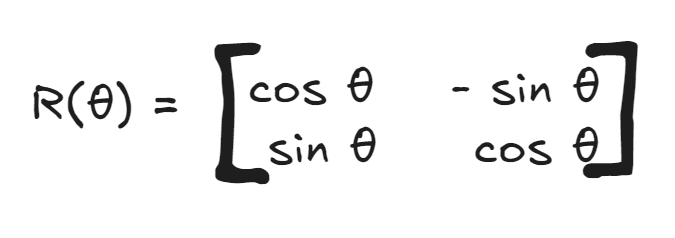
Therefore, for each token there will be 4 rotation matrices of shape (2,2). Finally each dimension pair value is multiplied with this rotation matrix and we obtain new pair of dimension values. To make this concept clear, here is visual flow shown just for token “the”.

Note:
Note: The values in Fig. 4 are arbitrary and used for conceptual understanding only. In practice, the 2*2 rotation matrix is not explicitly constructed for every dimension pair. Instead, the rotation is applied directly using:
x_even_new = x_even * cos θ — x_odd * sin θ
x_odd_new = x_even * sin θ + x_odd * cos θ
This is mathematically equivalent to the matrix multiplication shown above but computationally more efficient.
Pros:
1. Magnitude of token embeddings is fully preserved, no distortion since rotation doesn’t change vector length
2. Directly encodes relative distance, Q·Kᵀ dot product naturally depends only on (m-n), the distance between positions
3. Generalizes to longer sequences than seen during training, better than learned PE since it’s formula based
4. No additional parameters, like sinusoidal PE, nothing extra to train
5. Currently the standard in modern LLMs: LLaMA, Mistral, Falcon, Gemma all use RoPE
Cons:
1. More computationally complex than simply adding a positional vector
2. Extrapolation to very long sequences (far beyond training length) still degrades, addressed by variants like YaRN and LongRoPE but not solved in base RoPE
RoPE code implementation:
The implementation follows directly from the math. In __init__, all angles (position*frequency) are precomputed once and stored as a non-trainable buffer, no need to recompute every forward pass. In forward, Q or K is split into even and odd dimensions, the rotation formula is applied directly, and the pairs are interleaved back to restore the original shape.
class ApplyRoPE(nn.Module):
    def __init__(self, head_dim, context_length):
        super().__init__()
        i = torch.arange(0, head_dim, 2).float()
        freqs = 1.0 / (10000 ** (i / head_dim))
        pos = torch.arange(context_length).float()
        angles = pos.unsqueeze(1) * freqs.unsqueeze(0)  # [context_length, head_dim/2]
        self.register_buffer("angles", angles)
    def forward(self, x):
        # x shape: [batch, num_heads, seq_len, head_dim]
        seq_len = x.shape[2]

        # split into pairs
        x1 = x[..., 0::2]  # even dimensions [batch, heads, seq_len, head_dim/2]
        x2 = x[..., 1::2]  # odd dimensions  [batch, heads, seq_len, head_dim/2]

        # get cos and sin for current sequence length
        cos = torch.cos(self.angles[:seq_len, :])  # [seq_len, head_dim/2]
        sin = torch.sin(self.angles[:seq_len, :])  # [seq_len, head_dim/2]

        # apply rotation
        x1_new = x1 * cos - x2 * sin
        x2_new = x1 * sin + x2 * cos

        # interleave x1_new and x2_new back together
        x_rotated = torch.stack([x1_new, x2_new], dim=-1)
        x_rotated = x_rotated.flatten(-2)  # [batch, heads, seq_len, head_dim]

        return x_rotated.type_as(x)
This class is instantiated once inside MultiHeadAttention and called on both Q and K before the attention score computation. V is left untouched.
Positional embeddings have come a long way — from fixed sinusoidal formulas, to learned vectors, to rotation based encoding. Each approach addressed the limitations of the previous one. RoPE’s elegance lies in the fact that positional information is no longer something added on top — it is baked into the geometry of the attention mechanism itself. That is why it has become the default choice in almost every modern LLM built today.
The full implementation of this, along with the complete GPT-2 style LLM trained from scratch, is available on my GitHub repository.
References:
- Su, J., et al. (2021). RoFormer: Enhanced Transformer with Rotary Position Embedding. arXiv:2104.09864
- Vaswani, A., et al. (2017). Attention Is All You Need. arXiv:1706.03762
Understanding Positional Embeddings in Transformers (with Intuition and Examples) was originally published in Towards AI on Medium, where people are continuing the conversation by highlighting and responding to this story.