The complete guide to learning rate dynamics, batch configuration, scheduler calibration and overfitting detection.

While building Antijection, a prompt injection detection API, the first training run used hyperparameters thrown together without much thought. The model trained. The loss looked fine. The model was terrible.
That is the version of the story nobody talks about. The run completes, the numbers look reasonable, and the model fails in ways that only make sense in hindsight. Every hyperparameter in that config was a guess. Learning rate, batch size, epochs, weight decay, none of it was reasoned from first principles.
That is what this article fixes. Each major hyperparameter decision in a LoRA fine-tuning run has a derivable reason. By the end of this article, those reasons are all on the table, and nothing in the config is a guess anymore.
Table of Contents
- The Concentration Problem: Why LoRA Changes Everything About Learning Rate
- Effective Batch Size Is a Compound Variable
- The Scheduler Is Only As Good As Its Warmup
- Overfitting Happens Faster Than You Think, And Quietly
- train_on_responses_only Is Not a Trick, It’s Information Theory
- Precision, Seeding, and the Things That Fail Silently
Chapter 1: The Concentration Problem: Why LoRA Changes Everything About Learning Rate

In full fine-tuning, every parameter in the model is trainable. A 7-billion parameter model has 7 billion surfaces to absorb gradient pressure. When a loss signal arrives, it spreads across the entire weight space, and any single parameter receives only a tiny fraction of the total update force. This distribution acts as a buffer. It is why full fine-tuning is relatively tolerant of aggressive learning rates. The gradient energy dissipates across a massive area before it can do serious damage to any individual weight.
By freezing the base model and routing all learning through a pair of low-rank adapter matrices, the entire loss signal concentrates onto a fraction of the original parameter count. Unsloth’s documentation puts it directly, LoRA means optimizing roughly 1% of a model’s weights instead of all of them. The adapter receives the same magnitude of gradient signal that used to be spread across billions of parameters. Learning rate sensitivity in LoRA is not a matter of degree compared to full fine-tuning. It is a categorically different problem.
The practical consequence is specific. The recommended starting point for learning rate in a standard LoRA or QLoRA fine-tuning run is 2e-4, with the full workable range extending down to 5e-6 depending on the task and dataset. Exceeding 2e-4 by a meaningful margin does not produce a gradual performance penalty. It pushes the adapter weights out of the viable region of the loss landscape before the model has had any real opportunity to learn the target task. The updates are too violent for a parameter space that small. At the low end, dropping too far below the starting recommendation without good reason means the adapter barely moves from its initialization. The base model's behavior dominates, and the fine-tune produces a model indistinguishable from its starting point.
The rank-alpha relationship is not two independent knobs
Rank and alpha get treated as separate decisions in most tutorials. They are not. What actually enters the residual stream is the adapter output scaled by alpha / rank. That ratio is the effective injection strength. Setting rank to 16 and alpha to 16 produces a scaling factor of 1.0, which is conservative and stable. Setting alpha to 32 with the same rank doubles the injection strength, which accelerates adaptation but increases the risk of destabilizing the pre-trained residual representation.
The architectural reason this matters was covered in episode 1. Every transformer layer adds its sub-layer output to a persistent residual stream rather than replacing it. LoRA works by injecting its own update, the product AB, into that same stream. If the injected signal is too large relative to the existing residual, the pre-trained knowledge in the base model gets overwhelmed. The model starts forgetting what it already knew faster than it learns what the fine-tuning task requires.
Unsloth’s documentation states the recommendation clearly, set alpha equal to rank, or use r * 2 as a common heuristic. The first is the conservative default that preserves residual stream integrity. The second is a deliberate choice to accelerate learning. Both values need to be chosen together, with their ratio in mind, not independently.
What this means before writing a single line of config
Three facts determine the learning rate and alpha/rank decisions, the size of the adapter relative to the base model, which sets gradient sensitivity; the complexity of the task, which informs whether a conservative or aggressive alpha/rank ratio is warranted; and the dataset size, which affects how many gradient steps are available before overfitting risk climbs. None of these can be ignored in favor of a copied default.
An adapter pushed into an unusable region by an oversized learning rate in the first 300 steps cannot be rescued by better batch configuration or a well-tuned scheduler. Learning rate is the precondition everything else depends on.
Chapter 2: Effective Batch Size Is a Compound Variable

Learning rate sets the magnitude of each update. Effective batch size determines the quality of the gradient signal informing it. On the hardware constraints that most LoRA runs operate under, these two concerns collide in a way that is not obvious until the first OOM error.
per_device_train_batch_size vs gradient_accumulation_steps
These two parameters look like they control the same thing. They do not. per_device_train_batch_size controls how many training examples are processed in a single forward pass. That number determines VRAM consumption directly. gradient_accumulation_steps controls how many of those forward passes complete before a single weight update executes. That number determines wall-clock time per update, not memory.
Effective batch size is the product of both: per_device_train_batch_size * gradient_accumulation_steps. A configuration of batch size 2 with 8 accumulation steps produces an effective batch of 16. A configuration of batch size 16 with 1 accumulation step also produces an effective batch of 16. The optimizer sees identical gradient signal in both cases. The GPU sees very different memory pressure.
Why real batch size is forced to 1 or 2 on 16–24GB VRAM
VRAM consumption does not scale linearly with sequence length. It scales quadratically. The attention matrix at the core of every transformer layer must be computed for every pair of tokens in the sequence. A sequence of length 4,096 produces over 16 million attention scores per layer. At 8,192 tokens, that number reaches approximately 67 million scores per layer. The memory required to hold that matrix grows with the square of the input length, independent of model size.
On a single consumer GPU with 16 to 24GB of VRAM, once model weights are loaded, the remaining budget for the forward pass is tight. With a model occupying 10–14GB, a real batch size above 1 or 2 at non-trivial sequence lengths exhausts what remains. The OOM error in this situation is not a model size problem. It is an attention matrix problem.
This is the constraint gradient accumulation is designed to work around. By keeping the real batch at 1 or 2 and accumulating over multiple steps, the practitioner gets the gradient stability benefits of a larger effective batch without materializing more than a small batch in memory simultaneously.
Gradient accumulation as a temporal substitute for memory
Gradient accumulation is a hack, and a useful one. Instead of computing one large batch in parallel, it computes many small batches in sequence, accumulates their gradients, and then applies a single update as if the large batch had been processed together. The mathematical result is equivalent. The trade-off is time. More accumulation steps means more sequential forward passes before any weight update occurs, which extends wall-clock training time proportionally.
The gain in signal quality often justifies this cost. Smaller individual batches produce noisier gradient estimates. For LoRA runs where the adapter parameters are few and the loss signal is already concentrated, gradient noise from tiny batches can push adapter weights erratically. Accumulation reduces that erratic behavior without touching VRAM usage.
max_seq_length and the most common source of unnecessary memory waste
Sequence length is the highest-leverage parameter for memory management, and also the most commonly misconfigured. Setting max_seq_length to 2048 when the actual training data has a 95th percentile length of 512 tokens wastes the memory budget on attention matrices that will never be populated. That wasted memory directly reduces the real batch size that fits in VRAM, which either limits gradient quality or forces more accumulation steps.
The correct approach is to histogram the dataset lengths first, then set max_seq_length to the 95th or 99th percentile of that distribution. Not the theoretical maximum the model supports, not the largest example in the dataset. This misconfiguration is one of the primary sources of inefficiency in practice. A model fine-tuned with max_seq_length = 2048 on data whose 95th percentile is 512 tokens consumes four times the attention memory it needs on most examples, translating directly into a four-fold reduction in achievable real batch size and cascading into longer training runs and noisier gradients.
The stability of a run comes from the effective batch size, not the real batch size. On a single GPU, keeping the real batch at 1 or 2 and raising accumulation steps is the standard approach to get both VRAM headroom and gradient quality simultaneously.
Chapter 3: The Scheduler Is Only As Good As Its Warmup

Learning rate sets the update magnitude. Batch configuration determines gradient signal quality. What neither covers is how the learning rate should evolve across the full training run. That is the scheduler’s job, and the scheduler has a dependency that practitioners consistently underweight.
Why cosine decay is the default
Cosine decay starts at the target peak, holds near it through the early portion of training where the model is making its largest behavioral adjustments, then smoothly reduces toward near-zero by the end. High learning rates early allow fast movement through the loss landscape while the gradient signal is most informative. Low learning rates late allow the optimizer to settle into a precise minimum rather than oscillating around it.
The alternatives are worth understanding in contrast. Linear decay drops the learning rate at a constant rate, which means it reaches low values sooner and gives the model less time in the high-LR exploration phase. Constant learning rate with warmup holds the peak for the entire run after warmup completes, which is appropriate for very short runs where cosine decay barely has time to engage before the run ends.
The warmup period and why LoRA specifically needs it
Warmup is the phase where the optimizer increases the learning rate from near-zero up to its target peak. In full fine-tuning, warmup is useful but not critical. LoRA makes it load-bearing.
LoRA adapter weights begin in a randomized or near-zero state. They have no pre-trained knowledge to anchor them. When the first gradient updates arrive, the adapter is maximally sensitive to where those updates point. A learning rate that starts at the full target value on step one applies the same force to completely uninformed weights as it would to well-calibrated weights fifty steps later. The result is that initial high-magnitude gradients can push the adapter weights into a suboptimal basin before the decay schedule even begins. The model lands there and stays there.
This connects directly to the alpha/rank ratio from chapter 1. That ratio controls how much force the trained adapter injects into the residual stream. Warmup controls how much force hits the adapter itself during the first steps of training. Both matter for the same underlying reason, uncontrolled early gradient pressure on a small parameter space causes damage that subsequent training cannot undo.
When to use constant_with_warmup instead
Cosine decay requires a minimum run length to be meaningful. On very short runs, the cosine curve does not have enough range to produce a meaningful learning rate reduction. The schedule begins its descent almost immediately after warmup ends, and the model spends most of its training in a transitional low-LR phase rather than the high-LR exploration phase where actual learning happens. For runs this short, constant_with_warmup is more appropriate: it completes warmup, then holds the peak learning rate flat for the remainder, letting the optimizer work at full strength throughout.
AdamW vs paged_adamw_8bit
SGD has no adaptive learning rates. Every parameter receives the same scaled gradient. In LoRA, where a few million adapter parameters coexist alongside frozen billions, a global learning rate that works for the adapter would be wildly inappropriate for the base model if it were trainable. AdamW’s per-parameter adaptive learning rates handle this asymmetry automatically, which is why it is effectively the only viable optimizer for LoRA fine-tuning.
The memory cost of AdamW is why its 8-bit paged variant exists. Standard AdamW maintains two momentum vectors per parameter in 32-bit floating point. According to the bitsandbytes documentation, 8-bit optimizers reduce GPU memory for optimizer states by 75%, because going from 32-bit to 8-bit state storage is a 4x reduction. The paged variant adds CPU offloading, optimizer states page out to CPU RAM under VRAM pressure and page back in only when needed for a given update. The accuracy cost of 8-bit moment quantization is negligible for fine-tuning. Small quantization errors in the gradient history estimate produce correspondingly small perturbations in update direction, well within the noise level of stochastic training.
Chapter 4: Overfitting Happens Faster Than You Think, And Quietly
A structurally sound training run, with correctly configured learning rate, well-managed batch setup, and a properly calibrated scheduler, can still produce a useless model. Not because anything went wrong mechanically, but because training ran too long. Chapter 4 is about knowing when to stop.
Why LoRA models overfit faster than full fine-tuning
The same property that makes LoRA memory-efficient makes it overfit rapidly. A small parameter space under concentrated loss signal memorizes training examples fast. On a small, clean dataset, the adapter can absorb the training distribution in as few as one to three epochs. Past that point, the adapter is no longer learning the task. It is learning the specific phrasing, structure, and surface patterns of the training examples themselves.
This happens faster than expected because the dynamic is asymmetric. In full fine-tuning, memorization requires the entire weight space to shift toward the training data. In LoRA, only the adapter matrices need to shift, and they are small. The optimizer reaches a state of per-example memorization in far fewer gradient steps. There is no warning before this transition. The training loss does not change character. It keeps descending.
Train loss vs eval loss
Training loss measures how well the model predicts its own training data. In a LoRA run on a small dataset, this number decreases reliably regardless of whether the model is generalizing or memorizing. The two failure modes produce identical training loss curves.
Eval loss is the metric that actually carries information. Computed on a held-out split that the optimizer never touches, it measures whether the learned adapter weights generalize to examples the model has not seen. When training loss continues to fall while eval loss plateaus or rises, the model is overfitting. Without an eval split, this divergence is invisible.
Monitoring eval loss is not an optional component of the training loop. It is the primary signal for determining when to stop. Epoch count alone is insufficient because the relationship between epochs and memorization depends on dataset size, data diversity, and effective batch size, none of which are constant across runs.
EarlyStoppingCallback and what patience actually means
The HuggingFace Trainer, which Unsloth uses, provides EarlyStoppingCallback for automated training termination. The mechanism monitors eval loss at each evaluation point and halts training when the loss fails to improve for a specified number of consecutive evaluations. That number is the patience value.
Patience is a tolerance for plateau, not a quality dial. Setting it too low stops training at the first sign of a plateau, which may be transient noise. Setting it too high allows the run to continue past the optimal checkpoint, accumulating degradation the final model carries into production. A patience of 3 to 5 evaluations is a practical starting range, scaled to eval frequency.
Eval frequency calibration
eval_steps controls how often the held-out split is scored. Set it too infrequently and the overfitting inflection point passes undetected, leaving the model to degrade for potentially hundreds of steps. Set it too frequently and inference overhead on the eval split slows the run.
Evaluating every 10 to 20 percent of an epoch is a practical default that provides enough resolution to catch divergence without spending excessive compute on evaluation passes. Eval frequency and patience need to be set together. A patience of 3 evaluations at 5 percent per epoch catches overfitting much faster than the same patience at 20 percent. The goal is to detect the eval loss inflection point within a small enough window that early stopping triggers before significant degradation accumulates.
Weight decay as regularization in the low-rank context
Weight decay applies L2 regularization to the adapter matrices by penalizing large weight values. In full fine-tuning, this effect spreads across billions of parameters. In LoRA, the same force acts on a much smaller count, giving weight decay a proportionally larger relative effect on the adapter.
Unsloth’s documentation identifies 0.01 as a reliable starting value. Setting it higher actively fights the learning signal, where the optimizer simultaneously minimizes task loss and weight magnitudes, and at high values, regularization pressure dominates. The adapter learns slowly or not at all. Setting weight decay to zero removes this check and increases the likelihood of an overfit state where the adapter loses the breadth of the base model’s original knowledge.
Epoch control as the blunt instrument
Unsloth’s documentation identifies 1 to 3 epochs as the standard safe zone for most instruction-based datasets. For most tasks, training beyond 3 epochs offers diminishing returns and increases memorization risk regardless of other regularization settings.
Epoch count is a ceiling, not a substitute for eval monitoring. Early stopping with a proper eval split terminates the run at the right moment within that range. Without early stopping, capping epochs at 3 is a coarse safeguard against the worst outcomes, not a guarantee of the optimal stopping point. The two mechanisms work together where epochs set the outer bound, early stopping finds the actual optimum within it.
Chapter 5: train_on_responses_only Is Not a Trick, It’s Information Theory
Chapters 1 through 4 established how to configure the gradient signal and when to stop applying it. This chapter is about making every gradient step count as much as possible. The mechanism is train_on_responses_only, and the reason it works is not intuitive until the loss function is examined directly.
What happens when loss is computed on the full prompt-response sequence
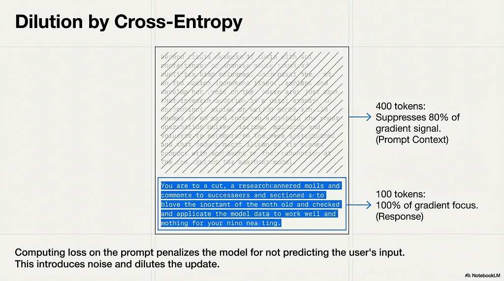
In a standard instruction fine-tuning setup, a training example consists of a prompt followed by a response. If cross-entropy loss is computed across all tokens in that sequence, the model is penalized at every position where it fails to predict the correct next token. That includes every token in the prompt.
The prompt tokens are inputs. The model received them as context. Computing loss on positions the model was given as known information forces the optimizer to spend gradient capacity on a task that cannot improve the model’s ability to generate useful outputs. Consider a concrete example: a training example with 400 prompt tokens and 100 response tokens. If loss is computed across all 500 tokens, 80 percent of the gradient signal at each step comes from positions where the model is penalized for not predicting the user’s input. The 20 percent of signal from the response tokens is diluted by a factor of four. The adapter learns something from every step, just not primarily what the task requires.
The information theory framing
Cross-entropy loss measures the negative log probability the model assigns to the correct token at each position. When prompt tokens are included, the loss incorporates surprise at positions where the correct answer was provided as input. That surprise carries no information about whether the adapter is becoming better at the target task. It is noise in the precise information-theoretic sense: it enters the gradient without increasing the signal-to-noise ratio of the update.
train_on_responses_only removes this noise by setting the label index for all prompt tokens to -100. The HuggingFace cross-entropy implementation ignores positions with label -100 during loss computation. Those tokens still exist in the input sequence and still participate in the key-value attention computation, so the model retains full context from the prompt. No gradient flows from prompt positions. Every gradient step is informed exclusively by how well the model predicted the response.
This approach produces cleaner gradients and typically faster convergence on the target task. Research into “Instruction Modeling” shows measurable improvements on benchmarks including MMLU when training is restricted to response tokens rather than the full sequence.
Chat template alignment, where this actually fails in practice
train_on_responses_only is straightforward in principle and fragile in implementation. The feature identifies which tokens belong to the prompt and which to the response by matching against the chat template delimiters used by the specific model being fine-tuned.
As we mentioned in the previous episode, every model family uses a different chat template. Llama 3 uses one set of special tokens to mark user and assistant turns. Qwen uses another. Mistral uses another. The instruction_part and response_part arguments passed to train_on_responses_only must match the exact delimiter tokens that the tokenizer produces for that model's template. If they do not, two failure modes are possible. The masking can fail to apply entirely, leaving the full sequence contributing to loss as if the feature were not enabled. Or the masking can apply incorrectly, removing gradient signal from response tokens that should be contributing it.
Task-specific guidance
Response-only training is the correct default for instruction-following, conversational, multi-turn reasoning, and classification tasks. In each of these, the output is what the adapter needs to learn, and the prompt is context that should inform but not penalize.
The one case where full-sequence training may be warranted is knowledge injection, where the goal is to make the model internalize factual associations from the training text rather than learn a specific output behavior. Here the prompt and response distinction is less meaningful, and masking the first portion of each example may remove useful learning signal. For classification tasks specifically, the benefit of response-only training is concentrated. The response is often a single token or short label sequence. Masking the prompt focuses the entire gradient budget of each step onto the relationship between the input context and that label.
Chapter 6: Precision, Seeding, and the Things That Fail Silently
The previous five chapters covered every major decision point in the training loop. Each of those decisions produces observable effects. This chapter covers the failure modes that produce none. The run completes cleanly. The metrics look reasonable. The model is broken in a way that only surfaces when it matters.
BF16 vs FP16, why the difference is not about precision
The intuitive framing of floating point formats is that higher precision means better results. That framing is wrong for LLM training, and the wrong choice creates one of the most opaque failure modes in practice.
BF16 and FP16 both use 16 bits per value, but they allocate those bits differently. FP16 uses 5 bits for the exponent and 10 bits for the mantissa. BF16 uses 8 bits for the exponent and 7 bits for the mantissa. BF16 matches FP32 exactly in its exponent range while sacrificing some numerical resolution. FP16 has higher resolution but a much narrower range of representable values.
For LLM training, the exponent range is what matters. Gradients during backpropagation span many orders of magnitude across layers and training steps. When a gradient value falls outside FP16’s representable range, it does not round to the nearest valid value. It underflows to zero. That gradient, and everything it was supposed to update, stops learning. This is the specific failure mode BF16 was designed to prevent. Its wider exponent range handles the full distribution of gradient magnitudes that deep transformer training produces.
The failure is silent because the loss curve does not necessarily reflect it. A model can lose gradient signal in specific layers while aggregate loss continues to decrease, driven by the layers still receiving valid updates. The output quality degradation shows up at inference, not during training.
BF16 requires Ampere-generation hardware or newer: the RTX 30 series, A100, and more recent GPUs. On older hardware including the Tesla T4 and V100, BF16 is not available. For these GPUs, FP16 with automatic mixed precision [AMP] and gradient scaling is the correct configuration. Gradient scaling artificially inflates gradient magnitudes before the backward pass and deflates them before the weight update, keeping values within FP16’s representable range. According to Unsloth’s troubleshooting documentation, choosing the wrong dtype for the hardware can produce a model that generates incoherent outputs despite a normal-looking training run. Unsloth handles dtype detection automatically in most cases, but verifying the configuration before the run is the correct practice.
What gradient underflow actually looks like
There is no error. There is no warning. The loss descends on a reasonable curve. The model generates text. The text is wrong in ways that suggest the model did not learn the fine-tuning task, but the failure is indistinguishable from underfitting unless the dtype configuration is checked directly.
This is the most frustrating category of training failure because it forecloses the normal debugging loop. If the loss curve is the diagnostic, and the loss curve looks fine, the investigation never reaches the actual cause. Verify the dtype stack before the run, not after an unexplained failure.
Seed and CUDA non-determinism
Setting a fixed random seed ensures consistent data shuffling and consistent weight initialization for the adapter matrices. These are what most practitioners assume a seed provides. What a fixed seed does not guarantee is bit-for-bit identical results.
Many low-level CUDA operations involve parallel reductions, where multiple threads write to the same memory address simultaneously. The order in which those writes arrive is not deterministic. Because floating-point addition is not associative, meaning (a + b) + c does not always equal a + (b + c) at the level of floating-point representation, different orderings of the same additions produce slightly different results. According to PyTorch's reproducibility documentation, this variance exists at the level of least significant bits and is inherent to parallel GPU computation.
For most fine-tuning tasks this micro-variance is acceptable. The differences between runs with the same seed are smaller than the noise introduced by stochastic gradient descent itself.
The situation changes during hyperparameter sweeps. When comparing two configurations to determine which produces better eval metrics, run-to-run variance from non-deterministic CUDA operations can make a genuinely better configuration appear worse on a given run due to initialization luck. Distinguishing a real improvement from favorable variance requires multiple runs per configuration.
True determinism is available via torch.use_deterministic_algorithms(True). The cost is significant, the flag disables the faster non-deterministic kernels that libraries like Unsloth rely on for their performance advantages. The practical approach for production runs is to use seeding for data shuffling and initialization consistency, and to treat CUDA micro-variance as a known property of GPU training rather than a problem requiring elimination. For hyperparameter comparison, run each configuration multiple times with different seeds and compare distributions rather than single runs.
Conclusion
Six chapters have covered the full lifecycle of hyperparameter decisions in a LoRA fine-tuning run. Learning rate sets the update magnitude relative to the concentrated gradient pressure of a small adapter, with 2e-4 as the recommended starting point for standard LoRA and QLoRA. Effective batch size and gradient accumulation trade memory for signal quality on constrained hardware. The cosine scheduler and warmup period control how the learning rate evolves from fragile early steps to confident late refinement. Eval monitoring, early stopping, weight decay, and epoch control determine when the run should end. Response-only training focuses every gradient step on the tokens that actually matter. Dtype selection and seed behavior determine whether the results are numerically valid and whether comparisons between runs carry meaning.
None of these decisions are independent. A well-configured scheduler with inadequate warmup still produces a bad start on small datasets. Response-only training with misaligned chat templates silently reverts to full-sequence training. Knowing each piece individually is what makes the interactions between them diagnosable. When a run fails, or produces a model that underperforms, the cause is somewhere in this space. Knowing the space is how the cause gets found.
Episode 5 goes into post-training, quantization formats, export strategies, and the inference infrastructure decisions that determine whether a well-trained model actually delivers on its latency and cost requirements in production.
Connect with me on LinkedIn: https://www.linkedin.com/in/suchitra-idumina/
Note — The primary purpose of the images (slides) is to provide intuition. As a result, some oversimplifications or minor inaccuracies may be present.
The LoRA Hyperparameters No One Explains | How to Fine-Tune Correctly, Part 4 was originally published in Towards AI on Medium, where people are continuing the conversation by highlighting and responding to this story.