This is a sequel to our previous post on the Touchette-Lloyd theorem[1]. The previous post contained some introductory material and motivation for the theorem. Here, we will walk through the proof of the theorem and explore its applications in a few worked examples. It isn't strictly necessary to read that post before this one, but we recommend it if anything in this post seems unclear or if you would like some more background.
Recap and Setup
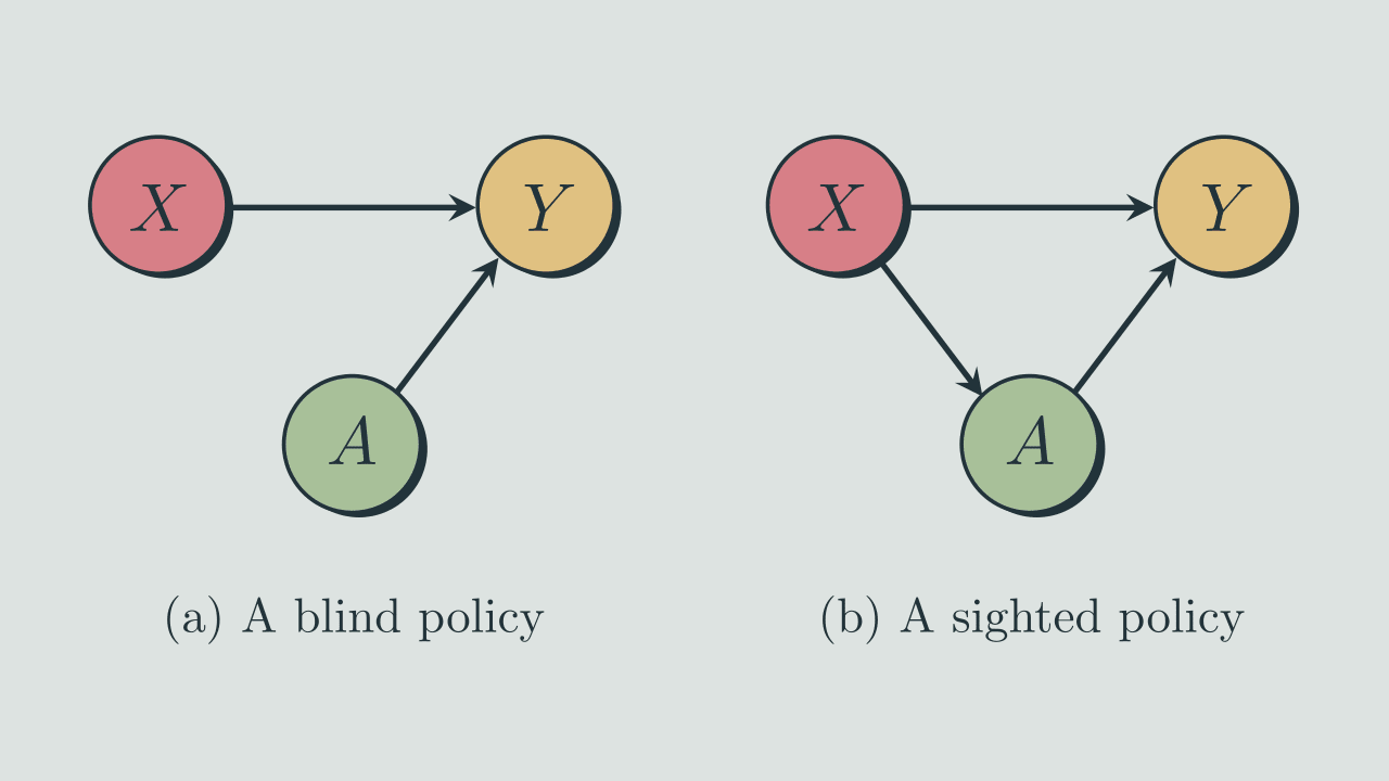
The theorem concerns three random variables. These are: the input 'environment' variable denoted by , the 'action' taken by a policy denoted by , and the output environment variable, denoted by . The environmental output is affected by the action and the initial environmental state. The way in which it is affected is given by expressed by a conditional probability distribution , which we will refer to as the 'dynamics' of the system. If is equal to either 0 or 1 for all values of then we will say that the dynamics is deterministic, but we will also allow for stochastic dynamics. As is standard, we will denote specific values that the random variables can take using lower case (eg. are values which can take, are values which can take). The variables and both represent the state of the 'environment' at different times (before and after the 'action' is taken). They will therefore both have the same domain (set of possible values) but we will nonetheless use (as opposed to ) to denote -values to avoid confusion over variables.
The way in which the action variable depends on the input environmental state is called the 'policy'. The theorem concerns the comparison of two classes of polices: 'Blind' policies where the action cannot depend on (or 'see') the environmental state and 'sighted' policies where the action taken can depend on . [2] These policies can be represented by Bayes nets:
The theorem statement is the inequality
which relates the entropy change for a sighted policy with mutual information between the environment and action to the maximum possible entropy change achievable for a blind policy .
The Proof
We will use the subscript to indicate a blind policy (so is the environmental output for a blind policy, is the action variable for a blind policy). First, let us look at what the output distribution looks like for a blind policy. The dynamics is fixed and and are independent so the probability distribution over will be
Let us consider the performance of a policy like this in producing a distribution with a low final entropy. In particular, we can quantify this using the difference between the initial environmental entropy and the final environmental entropy :
Quantifying entropy reduction in this way is intuitive and captures the fact that (other things being equal) it is more impressive for a agent or controller to achieve a low output entropy from a high starting entropy than to start with a low entropy and maintain it.
For any given initial distribution, there is a maximum which can be achieved using a blind policy, but depends on the initial distribution. Consider the set of all possible initial probability distributions , that is, all distributions over the state space containing , ... etc. For each there is a 'best' which can be achieved using a blind policy and cannot be surpassed by another blind policy acting on the same input distribution. Furthermore, there is some combination of initial distribution and policy which achieves a value of such that there is no other combination of blind policy and initial distribution which achieves a greater . Let this optimal value of achievable by a blind policy be labelled :
where is the set of all distributions over actions which correspond to blind policies.
We can ask: is there a combination of initial distribution and sighted policy which can outperform this value of ? And if so, by how much does it outperform this value? We will answer this question by investigating some general properties of sighted policies.
For a general 'sighted' policy, the action will depend on the environmental state , so the output distribution will include this dependency
Notice that we can use Bayes rule to re-write the conditional probabilities relating and . In particular, we can write
where
Note that this doesn't imply that the causal relationship between and has changed. We are still considering the case where the policy changes its action depending on what environmental state it 'sees'. We are just re-writing the probabilities.
Substituting this back in and rewriting the order of things, we can write the output distribution for a general policy as
Notice that this is a weighted average over probability distributions for each -value. If we consider only the cases where the action taken is one particular -value, say , we can obtain a conditional probability distribution over :
Interestingly, (and this is the key insight of the proof) we can think of this conditional output distribution for a sighted policy as the output distribution of a blind policy which always selects acting on an input distribution [3]. This means that the difference between the entropy of and is upper bounded by the blind policy entropy reduction . We can therefore write
Furthermore, since was arbitrary, this inequality holds for every possible -value, meaning that we can sum over the -values used by the sighted policy, weighted by :
This allows us to simplify this equation and obtain
To turn this bound on conditional entropies into a bound on for a general policy, we can add the entropy of the initial distribution to both sides and re-arrange to obtain:
Now, note two things. First, since , we can write
Second, note that , the difference between the entropy of and the entropy of , conditional on , is the definition of the mutual information between and so . Combining these two observations, we arrive at the following inequality relating the entropy reduction achievable through sighted policies to the blind entropy reduction:
which is the result!
What does this result tell us?
From the point of view of the agent structure problem, we can view this result as a selection theorem which tells us that, if we select for (or observe) a policy which achieves an entropy reduction which is greater than then, at minimum, its actions must share an amount of mutual information with the environment.
Examples of different dynamics
To gain some intuition for this result, we will explore its implications through a few examples. These can have very different feels, but in all cases, the dynamics are fully specified by defining the conditional distribution for all and .
1. Entropy decreasing dynamics
First, we will consider an entropy decreasing dynamics. In this example the entropy of the environment will naturally tend to decrease, without help from the policy. A simple example of such a dynamics is one where all input states are mapped to the same output, regardless of the action taken by the policy. If we consider each state to be labelled by a 5-bit string the following probability distribution has this property:
If we only observed environmental states, we would see that regardless of the entropy of the initial distribution over input strings, the output distribution would have zero entropy. Naively, one might attribute this entropy reduction to an effective policy using information about its environment. But in fact, the entropy reduction is a property of the environmental dynamics, not the policy. This can be seen by the fact that no policy, blind or sighted, can achieve a greater entropy change than that achieved by a blind policy. For this dynamics, , and no policy can achieve a greater entropy reduction. In this sense, tells us the the degree to which the environment itself contains entropy-reducing dynamics. We can see a slightly more subtle example of this by considering the following environmental dynamics
In words: the output state is equal to the input state, unless the action taken is , in which case the output state is . This dynamics contains two subdynamics: one (where ) which is entropy preserving and one (where ) which is entropy decreasing. A blind policy can guide the dynamics to become entropy decreasing (by picking ) and thus achieve maximal entropy reduction without requiring knowledge of the input state. In this sense, again captures the entropy-reducing qualities present in the environment itself, as opposed to the entropy-reducing qualities of a policy.
2. Entropy non-increasing dynamics
Let's return to the example given in the previous post, where the policy has to guess the correct 5-bit string. The dynamics of this example is deterministic and characterised by the following conditional probabilities
In words: the output state is if the action picked has the same string as the input state. Otherwise the output state is the same as the input state.
First, we will find . We do this by finding a blind policy and input distribution which maximizes the change in entropy between the input distribution and the output distribution. Note that the only way that a policy can reduce the entropy is to guess the correct string and that randomizing which string is guessed can do no better than picking the same (highest probability) string each time. Furthermore, the dynamics are symmetric with respect to all strings except 00000 so without loss of generality, we can assume that the best blind policy involves picking the string with probability one. Now, we need to find which input distribution maximizes for this policy.
First note that if is restricted to only having nonzero probabilities over and , then the final distribution will always have zero entropy. Therefore, in this restricted case, the maximum entropy reduction is achieved when the input distribution has maximum entropy (ie. which has 1 bit of entropy). This leads to an entropy reduction of 1 bit. We will now show that this distribution is in fact optimal and .
Note also that the above argument can be extended to show that, for any initial distribution, the blind policy will always achieve a greater entropy reduction when the probabilities of 00000 and 11111 are equal compared to when they are not.
Now, notice that any input distribution can be viewed as a mixture between a distribution over the domain which we will call and some other distribution over a domain not including 00000 and 11111 which we will call . Thus we can write the optimal input distribution as:
where is the optimal distribution over and is a 'mixing probability'. Since this distribution is a mixture of two distributions over non-overlapping domains, its entropy is given by:
where is the binary entropy of the mixing constant (a nice proof of this fact can be found here).
Now let us consider the output entropy for this distribution, under a blind policy. With probability , the output will be 00000, since any result in the domain will be mapped to 00000. We will call this outcome which has zero entropy so . With probability , the output will be a random variable from the distribution . The entropy of the total output can similarly be thought of as a mixture of non-overlapping distributions meaning that we can write it as
By subtracting from we can find the change in entropy between input and output:
The terms involving distributions over the domain excluding cancel out. Therefore, the blind entropy reduction is maximized by setting and as a maximum entropy distribution over the domain. We have therefore proved that . This means that if we observe a policy achieving an entropy reduction of greater than 1 bit on some input policy, we know that policy must be sighted-its actions must have some mutual information with the environmental state. In practice, this means that the policy must be taking in information about the environmental state.
Suppose we now observed a policy which achieved an output entropy of 2.83 bits when fed a maximum entropy input distribution with bits. Armed with the Touchette-Lloyd theorem, what can we deduce about this policy?
The entropy reduction achieved by this policy is bits. Since the inequality tells us
this means that our policy must have at least bits of mutual information with the environment. In fact, the policy which achieves this entropy change is the policy described in the first post, in the section titled 'A Formal Example'. This policy takes the first four bits of the environmental state (and then selects the action where are the first four bits of ) and thus has four bits of mutual information. This example raises an important point about the Touchette-Lloyd inequality which is that while it is true (4 bits is indeed greater than 1.17 bits) it doesn't always saturate. It would be nice if we could get a higher lower bound on the mutual information. There are two related ways to use the inequality to tighten the bound.
First, note that in the derivation of the inequality, we used the fact that , so unless we have a situation where , we cannot expect the bound to be tight. In a step near the end of our derivation, we obtained the inequality
Since , we can use this to obtain a tighter bound:
In our case, while , we have . This is because we can tell the first four bits of by looking at . For a uniform input distribution, given , the probability and . Using and yields the improved bound
So in fact, we can improve on the bound provided by the original Touchette-Lloyd inequality, provided that we are willing to replace with the slightly less intuitive quantity . However, the advantage of using the inequality in terms of is that knowing involves only observing changes in the environment and does not presume knowing all the actions which the policy takes. After all, if you already know what actions a policy is taking, you can probably calculate the mutual information already. From a selection theorem point of view we are more interested in inferring that a policy is using information from its environment by observing the changes in the environment.
Another way to increase the lower bound on is to observe the policy for different initial distributions. For example, if the policy was run on a distribution which was uniform over all 5-bit strings which end in '1' then the initial entropy would be bits but the policy would reduce the final entropy to , achieving . When plugged into the Touchette-Lloyd inequality (along with ) this would give a lower bound of 3 bits on the mutual information which is much tighter than the 'unoptimized' value of 1.17 bits (recall, the true mutual information between the action and environment for this policy is 4 bits).
3. Entropy increasing dynamics
We described the dynamics above as 'entropy non-increasing', since it is impossible for any policy to lead to an output distribution with a higher entropy than the input. We can also consider dynamics where entropy can increase and a policy has to be more proactive in fighting this entropy increase.
Consider the following dynamics, again in a situation where both environmental state and the action are described by 5-bit strings. If the action matches the environmental state (ie. if ), then the output environmental state is . On the other hand, if the action does not match the state (ie. if ) then is drawn from a uniform distribution over all 5-bit strings excluding 00000. This has dynamics corresponding to the following distribution
Using a similar argument to the one in the previous section, we can find that the maximum blind policy entropy change is 0 bits, achieved when the initial distribution (and the corresponding action string) is completely concentrated on one environmental state. This is because any initial distribution which allows the policy to guess wrong will be punished by a high-entropy final state leading to a negative .
Consider the sighted policy from the previous section which can 'see' the first four bits and chooses the action in this new environment. For a uniform initial distribution, this leads to a final distribution with and for strings . This output distribution has an entropy of so , leading to the lower bound on the entropy of .
Similarly to the previous section, we can improve on this bound by changing the initial distribution. If we consider the case where the initial distribution is over all strings which end in the bit '1' then this sighted policy chooses the correct action every time and reduces the final entropy to zero. This corresponds to . Since , this gives us the bound . Recall that this policy does indeed have 4 bits of mutual information with the environment, so this bound cannot be improved upon.
Moving to an environment which was more hostile to entropy reduction leads to a greater discrepancy between blind and sighted policies, this in turn allows the bound on mutual information provided by the Touchette-Lloyd inequality to be made tighter than in the 'entropy non-increasing' environment of the previous example.
Incidentally, this environment also highlights why, when calculating , the maximum must be taken over all initial distributions. It would be convenient if the inequality was true but was instead defined as the maximum change in entropy achievable for a blind policy with the same initial distribution as the term in the inequality. But this is not the case, instead is defined as the maximum entropy change achievable for a blind policy over any initial distribution. We can see why this must be the case by considering this environment.
If the initial distribution has intermediate entropy (ie. nonzero but not maximal) , then a sighted policy can achieve a zero entropy final distribution if it has full knowledge of the environmental state, meaning . A blind policy acting on this initial distribution will, most of the time guess the incorrect action to take, leading to the final state being drawn from an almost maximum entropy distribution. This can lead to the maximum blind policy entropy change being negative, (ie. the final distribution has a larger entropy than the initial distribution) for intermediate entropy distributions. If we define to be the maximum entropy change for a blind policy acting on an initial distribution and consider the for a sighted policy acting on the same initial distribution we might conjecture the following inequality
(NOTE: THIS INEQUALITY IS NOT TRUE!)
But we have just argued that a sighted policy can achieve using mutual information and that can be negative for the same initial distribution. Therefore the above inequality cannot hold.
On the other hand, if we define in the way that Touchette and Lloyd do, as the maximum blind entropy change achievable over all input distributions, then we can note that for a zero entropy initial distribution (ie. one where only takes a single value), a blind policy can achieve a zero entropy output distribution by choosing the correct action 100% of the time. This means that while was negative will equal zero, making the inequality valid. Understanding the slightly unintuitive way that is defined is important for using the Touchette-Lloyd theorem. We highlight this here as it was something that we took a long time to properly appreciate.
Conclusions & Further Work
We hope that the Touchette-Lloyd theorem is clear to you after reading this. We think that it is pretty interesting result from an Agent Foundations point of view and are interested in seeing if we can extend it. We have some ideas for a few avenues for further research.
Re-frame the result using expected utility. Reducing entropy and maximizing expected utility are (in some regards) similar in that they are both forms of optimization. If one policy achieves a particular expected utility (for some utility function over ) can we ascribe some lower bound on the mutual information between its actions and the environmental state?
Extend the result to a non-Markovian environment. We assumed here that the environment was Markovian so that X could be treated as a random variable independent of its previous value. But most interesting environments do not have this property. Does a similar result hold when a policy must 'remember' previous environmental states to choose optimally at a given timestep?
Policies which 'model' the dynamics, not just the state. The Touchette-Lloyd theorem broadly tells us when a policy has 'knowledge' of the environmental state. But having mutual information between the state and does not necessarily imply successful entropy reduction. In order to successfully reduce entropy, one must also choose actions which are appropriate for the dynamics of the environment. Can we prove a similar which captures whether a policy is modelling the dynamics of the system?
Prove an equivalent result using K-complexity. Entropy reduction is one hallmark of an optimizer. But if a system reduces in complexity or description length, it could also reasonably be said to be 'being optimized'. Can we prove a similar theorem involving the reduction of K-complexity, instead of entropy?
In control theory terminology, these families of policies are known as 'open loop' and 'closed loop' respectively. But as a personal preference we find the names 'blind' and 'sighted' more evocative so we will use them instead.
Touchette and Lloyd describe this as "the fact that a closed-loop controller is formally equivalent to an ensemble of open-loop controllers acting on the conditional supports instead of " (where they are using to represent a specific controller action, equivalent to our )