Sequence Modeling with CTC
A visual guide to Connectionist Temporal Classification, an algorithm used to train deep neural networks in speech recognition, handwriting recognition and other sequence problems.
A visual guide to Connectionist Temporal Classification, an algorithm used to train deep neural networks in speech recognition, handwriting recognition and other sequence problems.
<!–
–>
<!–
–>
<!–
–>
<!–Evolved Biped Walker.
–>
Going for a ride.
GitHub
In the previous article, I have described a few evolution strategies (ES) algorithms that can optimise the parameters of a function without the need to explicitly calculate gradients. These algorithms can be applied to reinforcement learning (RL) problems to help find a suitable set of model parameters for a neural network agent. In this article, I will explore applying ES to some of these RL problems, and also highlight methods we can use to find policies that are more stable and robust.
While RL algorithms require a reward signal to be given to the agent at every timestep, ES algorithms only care about the final cumulative reward that an agent gets at the end of its rollout in an environment. In many problems, we only know the outcome at the end of the task, such as whether the agent wins or loses, whether the robot arm picks up the object or not, or whether the agent has survived, and these are problems where ES may have an advantage over traditional RL. Below is a pseudo-code that encapsulates a rollout of an agent in an OpenAI Gym environment, where we only care about the cumulative reward:
def rollout(agent, env):
  obs = env.reset()
  done = False
  total_reward = 0
  while not done:
    a = agent.get_action(obs)
    obs, reward, done = env.step(a)
    total_reward += reward
  return total_reward
We can define rollout to be the objective function that maps the model parameters of an agent into its fitness score, and use an ES solver to find a suitable set of model parameters as described in the previous article:
env = gym.make('worlddomination-v0')

# use our favourite ES
solver = EvolutionStrategy()

while True:

  # ask the ES to give set of params
  solutions = solver.ask()

  # create array to hold the results
  fitlist = np.zeros(solver.popsize)

  # evaluate for each given solution
  for i in range(solver.popsize):

    # init the agent with a solution
    agent = Agent(solutions[i])

    # rollout env with this agent
    fitlist[i] = rollout(agent, env)

  # give scores results back to ES
  solver.tell(fitness_list)

  # get best param & fitness from ES
  bestsol, bestfit = solver.result()

  # see if our task is solved
  if bestfit > MY_REQUIREMENT:
breakOur agent takes the observation given to it by the environment as an input, and outputs an action at each timestep during a rollout inside the environment. We can model the agent however we want, and use methods from hard-coded rules, decision trees, linear functions to recurrent neural networks. In this article I use a simple feed-forward network with 2 hidden layers to map from an agent’s observation, a vector , directly to the actions, a vector :
The activation functions , can be tanh, sigmoid, relu, or whatever we want to use. In all of my experiments I use tanh. For the output layer, sometimes we may want to be a pass-through function without nonlinearities. If we concatenate all the weight and bias parameters into a single vector called , we see that the above neural network is a deterministic function . We can then use ES to find a solution using the search loop described earlier.
But what if we don’t want our agent’s policy to be deterministic? For certain tasks, even as simple as rock-paper-scissors, the optimal policy is a random action, so we want our agent to be able to learn a stochastic policy. One way to convert into a stochastic policy is to make random. Each model parameter can be a random value drawn from a normal distribution .
This type of stochastic network is called a Bayesian Neural Network. A Bayesian neural network is a neural network with a prior distribution on its weights. In this case, the model parameters we want to solve for, are the set of and vectors, rather than the weights . During each forward pass of the network, a new is drawn from . There are lots of interesting works in the literature applying Bayesian networks to many problems, and also addressing many challenges of training these networks. ES can also be used to directly find solutions for a stochastic policy by setting the solutions space be and , rather than .
Stochastic policy networks are also popular in the RL literature. For example, in the Proximal Policy Optimization (PPO) algorithm, the final layer is a set of and parameters and the action is sampled from . Adding noise to parameters are also known to encourage the agent to explore the environment and escape from local optima. I find that for many tasks where we need an agent to explore, we do not need the entire to be random – just the bias is enough. For challenging locomotion tasks, such as the ones in the roboschool environment, I often need to use ES to find a stochastic policy where only the bias parameters are drawn from a normal distribution.
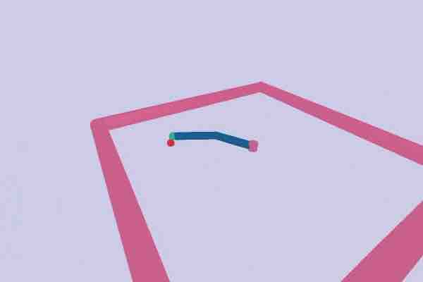
One of the areas where I found ES useful is for searching for robust policies. I want to control the tradeoff between data efficiency, and how robust the policy is over several random trials. To demonstrate this, I tested ES on a nice environment called BipedalWalkerHardcore-v2 created by Oleg Klimov using the Box2D Physics Engine, the same physics engine used in Angry Birds.
<!–
Our agent solved BipedalWalkerHardcore-v2.
–>
Evolution Strategy Variant + OpenAI Gym pic.twitter.com/t2R0QQ5qcH
— hardmaru (@hardmaru) July 23, 2017
Our agent solved BipedalWalkerHardcore-v2.
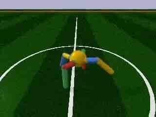
In this environment our agent has to learn a policy to walk across randomly generated terrain within the time limit without falling over. There are 24 inputs, consisting of 10 lidar sensors, angles and contacts. The agent is not given the absolute coordinates of where it is on the map. The action space is 4 continuous values controlling the torques of its 4 motors. The total reward calculation is based on the total distance achieved by the agent. Generally, if the agent completes a map, it will get score of 300+ points, although a small amount of points will be subtracted based on how much motor torque was applied, so energy usage is also a constraint.
BipedalWalkerHardcore-v2 defines solving the task as getting an average score of 300+ over 100 consecutive random trials. While it is relatively easy to train an agent to successfully walk across the map using an RL algorithm, it is difficult to get the agent to do so consistently and efficiently, making this task an interesting challenge. To my knowledge, my agent is the only solution known to solve this task so far (as of October 2017).
 Early stages. Learning to walk. |
 Learns to correct errors, but still slow … |
Because the terrain map is randomly generated for each trial, sometimes we may end up with an easy terrain, or sometimes a very difficult terrain. We don’t want our natural selection process to allow agents with weak policies who had gotten lucky with an easy map to advance to the next generation. We also want to give agents with good policies a chance to redeem themselves. So what I ended up doing, is to define an agent’s episode, as the average of 16 random rollouts, and use the average of the cumulative rewards over 16 rollouts as its fitness score.
Another way to look at this is to see that even though we are testing the agent over 100 trials, we usually train it on single trials, so the test-task is not the same as the training-task we are optimising for. By averaging each agent in the population multiple times in a stochastic environment, we narrow the gap between our training set and the test set. If we can overfit to the training set, we might as well overfit to the test set, since that’s an okay thing to do in RL 🙂
Of course, the data efficiency of our algorithm is now 16x worse, but the final policy is a lot more robust. When I tested the final policy over 100 consecutive random trials, we got an average score of over 300 points required to solve this environment. Without this averaging method, the best agent can only obtain an average score of 220 to 230 over 100 trials. To my knowledge, this is the first solution that solves this environment (as of October 2017).

|

|
Winning solutions evolved using PEPG using average-of-16 runs per episode.
I also used PPO, a state-of-the-art policy gradient algorithm for RL, and tried to tune it to the best of my ability to perform well on this task. In the end, I was only able to get PPO to achieve average scores of 240 to 250 over 100 random trials. But I’m sure someone else will be able to use PPO or another RL algorithm to solve this environment in the future. (Please let me know if you do so!)
Update (Jan 2018): dgriff777 was able to use a continuous version of A3C+LSTM with 4 stack frames as the input to train BipedalWalkerHardcore-v2 to obtain a score of 300 over 100 random trials. He provided this awesome implementation of his pytorch model on GitHub.
The ability to control the tradeoff between data efficiency and policy robustness is quite powerful, and useful in the real world where we need safe policies. In theory, with enough compute, we could have even averaged over of the required 100 rollouts and optimised our Bipedal Walker directly to the requirements. Professional engineers are often required to have their designs satisfy specific Quality Assurance guarantees and meet certain safety factors. We need to be able to take into account such safety factors when we train agents to learn policies that may affect the real world.
Here are a few other solutions that ES discovered:
 CMA-ES solution |
 OpenAI-ES solution |
I also trained the agent with a stochastic policy network with high initial noise parameters, so the agent sees noise everywhere, and even its actions are noisy. It resulted in the agent learning the task despite not being confident of its input and outputs being accurate (this agent couldn’t get a score of 300+ though):
<!–
–>
<!–
–>

<!–
–>
Bipedal walker using a stochastic policy.
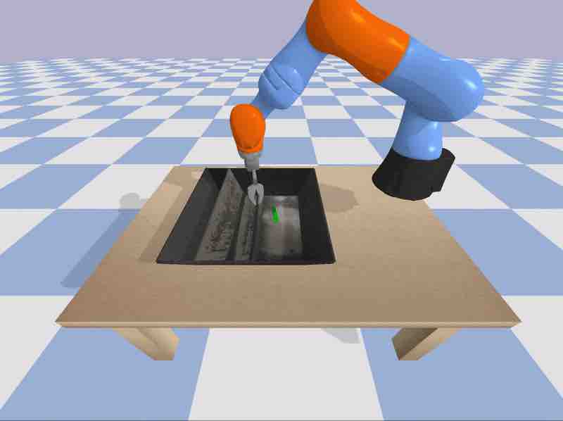
I also tried to apply ES with this averaging technique on a simplified Kuka robot arm grasping task. This environment is available in the pybullet environment. The Kuka model used in the simulation is designed to be similar to a real Kuka robot arm. In this simplified task, the agent is given the coordinates of the object.
More advanced RL environments may require the agent to infer an action directly from pixel inputs, but we could in principle combine this simplified model with a pre-trained convnet that gives us an estimate of the coordinates as well.
<!–
–>
<!–
–>
<!––>
Robot arm grasping task using a stochastic policy.
The agent obtains a score of 10000 if it successfully picks up the object, and 0 otherwise. Some points are deducted for energy usage. By averaging a sparse reward over 16 random trials, we can get the ES to optimise for robustness. However, in the end, I was able to get policies that can pick up the object only 70 to 75% of the time with both deterministic and stochastic policies. There is still room for improvement.
Learning to perform multiple difficult tasks at the same time make us better at performing individual tasks. For example, Shaolin monks who lift weights while standing on a pole will be able to balance better without the weights. Learning to not spill a cup of water while cruising a car at 80mph in the mountains will make the driver a better illegal street racer. We can also train agents to perform multiple tasks to make them learn more stable policies.
<!– –> –> <!––> Shaolin Agents. |
<!– –> –> Learning to drift. |
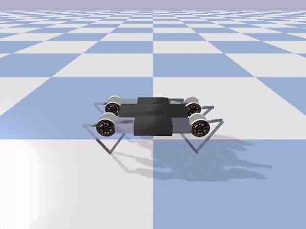
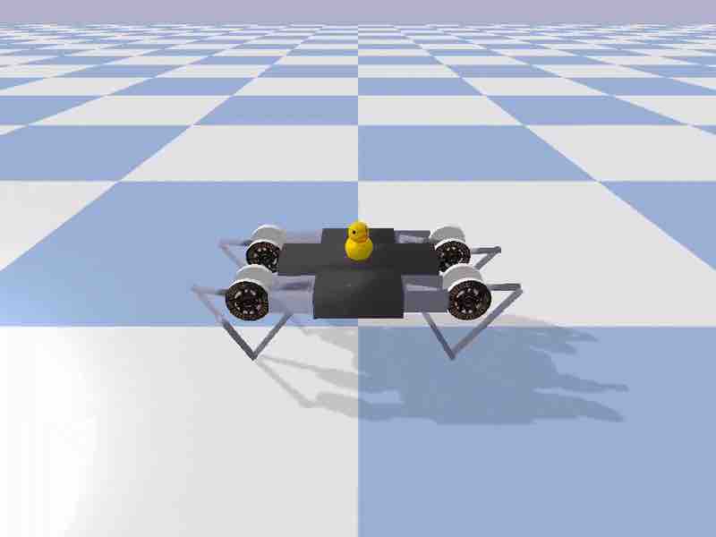
This recent work on self-playing agents demonstrated that agents who learn difficult tasks such as Sumo wrestling (a sport that require many skills) are able to also perform easier tasks, like withstanding wind while walking, without the need for further training. Erwin Coumans recently tried to experiment with adding a duck on top of a Minitaur learning to walk ahead. If the duck fell, the Minitaur would also fail, so the hope is that these types of task augmentation will help transfer learned policies from simulation over to the real Minitaur. I took one of his examples and experimented with training the Minitaur and duck combination using ES.
<!– –> –> <!––> CMA-ES walking policy in pybullet. |
<!– –> –> <!––> Real Minitaur from Ghost Robotics. |
The Minitaur model in pybullet is designed to mimic the real physical Minitaur. However, a policy trained on a perfect simulation environment usually fails in the real world. It may not even generalise to small augmentations of the task inside the simulation. For example, in the figure above is a Minitaur trained to walk ahead (using CMA-ES), but we see that this policy is not always able to carry a duck across the room when we put a duck on top of it inside of the simulation.
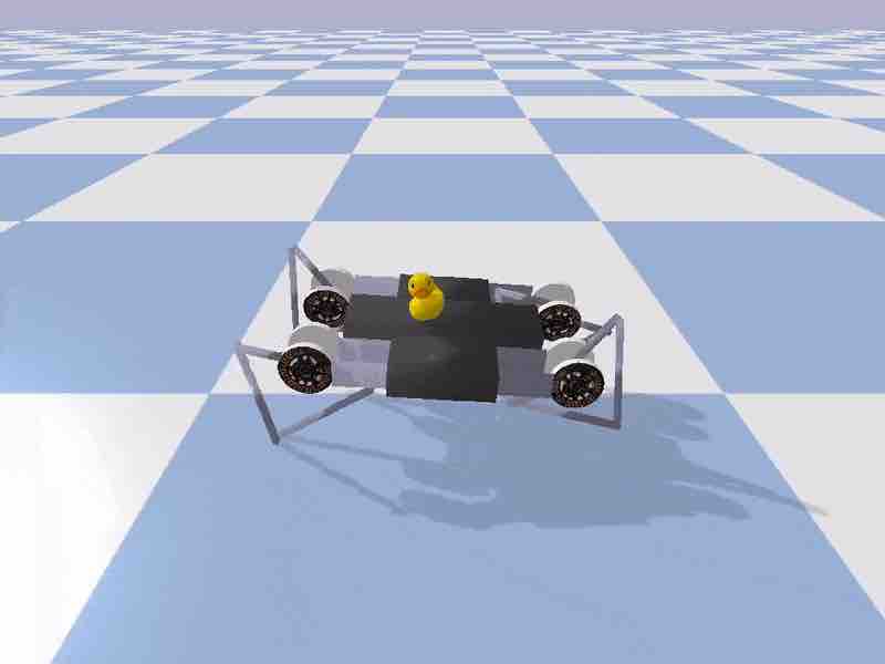 <!–  –> –><!––> Walking policy works with duck. |
<!––> Policy trained on duck. |
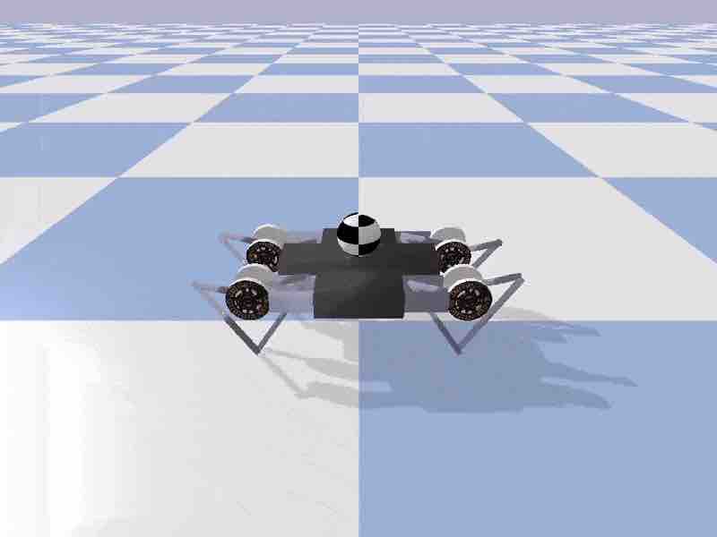
The policy learned from the pure walking task still works to some degree even when the duck is deployed, meaning that the addition of the duck wasn’t so difficult. The duck has a flat stable bottom so it wasn’t too difficult for the Minitaur to keep the duck from falling off its back. I tried to replace the duck with a ball to make the task much harder.
<!–
–>
<!–
–>
<!––>
Learning to cheat.
However, replacing the duck with a ball didn’t immediately result in a stable balancing policy. Instead, CMA-ES found a policy that still technically carried the ball across the floor by first having the ball slide into a hole made for its legs, and then carrying the ball inside this hole. The lesson learned here is that an objective-driven search algorithm will learn to take advantage of any design flaws in the environment and exploit them to reach its objective.
<!– –> –> <!––> Stochastic policy trained with ball. |
<!– –> –> <!––> Same policy with duck. |
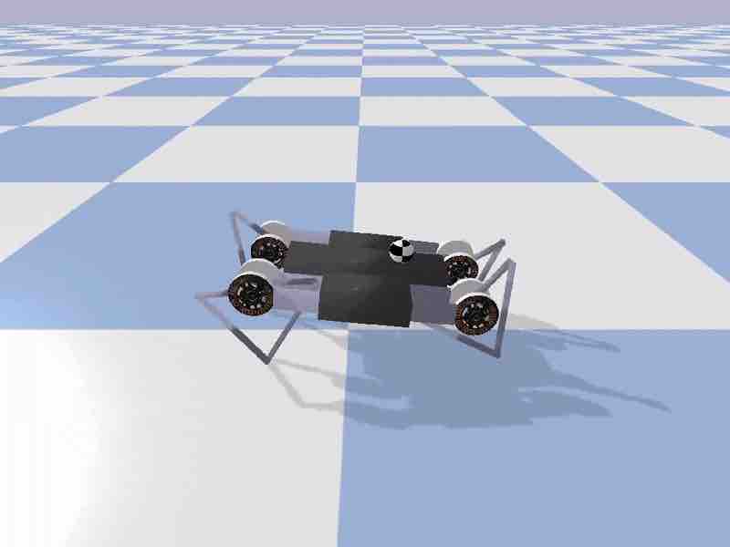
After making the ball smaller, CMA-ES was able to find a stochastic policy that can walk and balance the ball at the same time. This policy also transferred back to the easier duck task. In the future, I hope these type of task augmentation techniques will be useful for transfer learning to real robots.
One of the big selling points of ES is that it is easy to parallelise the computation using several workers running on different threads on different CPU cores, or even on different machines. Python’s multiprocessing makes it simple to launch parallel processes. I prefer to use Message Passing Interface (MPI) with mpi4py to launch separate python processes for each job. This allows us to get around the global interpreter lock, and also gives me confidence that each process has its own sandboxed numpy and gym instances which is important when it comes to seeding random number generators.
<!– –> –> <!––> Roboschool Hopper, Walker, Ant. |
 <!––> Roboschool Reacher. |
Agents evolved using estool on various roboschool tasks.
I have implemented a simple tool called estool that uses the es.py library described in the previous article to train simple feed-forward policy networks to perform continuous control RL tasks written with a gym interface. I have used estool tool to easily train all of the experiments described earlier, as well as various other continuous control tasks inside gym and roboschool. estool uses MPI for distributed processing so it shouldn’t require too much work to distribute workers over multiple machines.
In addition to the environments that come with gym and roboschool, estool works well with most pybullet gym environments. It is also easy to build custom pybullet environments by modifying existing environments. For example, I was able to make the Minitaur with ball environment (in the custom_envs directory of the repo) without much effort, and being able to tinker with the environment makes it easier to try out new ideas. If you want to incorporate 3D models from other software packages like ROS or Blender, you can try building new and interesting pybullet environments and challenge others to try to solve them.
Many models and environments in pybullet, such as the Kuka robot arm and the Minitaur, are modelled to be similar to the real robot as part of current exciting transfer learning research efforts. In fact, many of these recent cutting edge research papers are using pybullet to conduct transfer learning experiments.
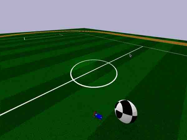
You don’t need an expensive Minitaur or Kuka robot arm to play with sim-to-real experiments though. There is a racecar model inside pybullet that is modelled after the MIT racecar open source hardware kit. There’s even a pybullet environment that mounts a virtual camera onto the virtual racecar to give the agent a virtual pixel screen as an input observation.
Let’s try the easier version first, where the racecar simply needs to learn a policy to move towards a giant ball. In the RacecarBulletEnv-v0 environment, the agent gets the relative coordinates of the ball as an input, and outputs continuous actions that control the motor speed and steering direction. The task is simple enough that it only takes 5 minutes (50 generations) on a 2014 Macbook Pro (with an 8-core CPU) to train. Using estool, the command below will launch the training job on eight processes and assign each process 4 jobs, to get a total of 32 workers, using CMA-ES to evolve the policies:
python train.py bullet_racecar -o cma -n 8 -t 4
The training progress, as well as the model parameters found will be stored in the log subdirectory. We can run this command to visualise an agent inside the environment using the best policy found:
python model.py bullet_racecar log/bullet_racecar.cma.1.32.best.json
<!–
–>
<!–
–>
<!––>
pybullet racecar environment, based on the MIT Racecar.
In the simulation, we can use the mouse cursor to move the ball around, and even move the racecar around if we want to interact with it.
The IPython notebook plot_training_progress.ipynb can visualise the training history per generation of the racecar agents. At each generation, we can see the best score, the worse score, and the average score across the entire population.


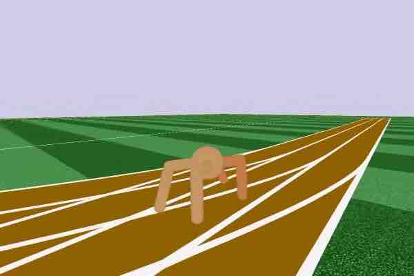
Standard locomotion tasks similar to those in roboschool, such as Inverted Pendulum, Hopper, Walker, HalfCheetah, Ant, and Humanoid are also available in pybullet. I found a policy for pybullet’s ant that gets to a score of 3000 within hours on a multi-core machine with a population size of 256, using PEPG:
python train.py bullet_ant -o pepg -n 64 -t 4
|
<!– |
<!– –> –> <!––> |
Example rollout of AntBulletEnv. We can still save rollouts as an .mp4 video using gym.wrappers.Monitor

In this article, I discussed using ES to find policies for a feed-forward neural network agent to perform various continuous control RL tasks defined by a gym environment interface. I described the estool that allowed me to quickly try different ES algorithms with various settings in a distributed processing environment using the MPI framework.
So far, I have only discussed methods for training an agent by having it learn a policy from trial-and-error in the environment. This form of training from scratch is referred to as model-free reinforcement learning. In the next article (if I ever get to writing it), I will discuss more about model-based learning, where our agent will learn to exploit a previously learned model to accomplish a given task. And yes, I will still be using evolution.
If you find this work useful, please cite it as:
@article{ha2017evolving,

  title   = "Evolving Stable Strategies",

  author  = "Ha, David",

  journal = "blog.otoro.net",

  year    = "2017",

  url     = "https://blog.otoro.net/2017/11/12/evolving-stable-strategies/"

}
I want to thank Erwin Coumans for writing all these great environments, and also for helping me work on making
ESTool better. Great research cannot be done without great tools.
In the end, it all comes to choices to turn stumbling blocks into stepping stones.
“Fires of a Revolution” Incredible Fast Piano Music (EPIC)
A Visual Guide to Evolution Strategies
Stable or Robust? What’s the Difference?
Evolution Strategies as a Scalable Alternative to Reinforcement Learning
Edward, A library for probabilistic modeling, inference, and criticism
History of Bayesian Neural Networks
Survival of the fittest.
<!–
Evolved Bipedal Walker
GitHub
–>
In this post I explain how evolution strategies (ES) work with the aid of a few visual examples. I try to keep the equations light, and I provide links to original articles if the reader wishes to understand more details. This is the first post in a series of articles, where I plan to show how to apply these algorithms to a range of tasks from MNIST, OpenAI Gym, Roboschool to PyBullet environments.
Neural network models are highly expressive and flexible, and if we are able to find a suitable set of model parameters, we can use neural nets to solve many challenging problems. Deep learning’s success largely comes from the ability to use the backpropagation algorithm to efficiently calculate the gradient of an objective function over each model parameter. With these gradients, we can efficiently search over the parameter space to find a solution that is often good enough for our neural net to accomplish difficult tasks.
However, there are many problems where the backpropagation algorithm cannot be used. For example, in reinforcement learning (RL) problems, we can also train a neural network to make decisions to perform a sequence of actions to accomplish some task in an environment. However, it is not trivial to estimate the gradient of reward signals given to the agent in the future to an action performed by the agent right now, especially if the reward is realised many timesteps in the future. Even if we are able to calculate accurate gradients, there is also the issue of being stuck in a local optimum, which exists many for RL tasks.

Stuck in a local optimum.
A whole area within RL is devoted to studying this credit-assignment problem, and great progress has been made in recent years. However, credit assignment is still difficult when the reward signals are sparse. In the real world, rewards can be sparse and noisy. Sometimes we are given just a single reward, like a bonus check at the end of the year, and depending on our employer, it may be difficult to figure out exactly why it is so low. For these problems, rather than rely on a very noisy and possibly meaningless gradient estimate of the future to our policy, we might as well just ignore any gradient information, and attempt to use black-box optimisation techniques such as genetic algorithms (GA) or ES.
OpenAI published a paper called Evolution Strategies as a Scalable Alternative to Reinforcement Learning where they showed that evolution strategies, while being less data efficient than RL, offer many benefits. The ability to abandon gradient calculation allows such algorithms to be evaluated more efficiently. It is also easy to distribute the computation for an ES algorithm to thousands of machines for parallel computation. By running the algorithm from scratch many times, they also showed that policies discovered using ES tend to be more diverse compared to policies discovered by RL algorithms.
I would like to point out that even for the problem of identifying a machine learning model, such as designing a neural net’s architecture, is one where we cannot directly compute gradients. While RL, Evolution, GA etc., can be applied to search in the space of model architectures, in this post, I will focus only on applying these algorithms to search for parameters of a pre-defined model.

Two-dimensional Rastrigin function has many local optima (Source: Wikipedia).
The diagrams below are top-down plots of shifted 2D Schaffer and Rastrigin functions, two of several simple toy problems used for testing continuous black-box optimisation algorithms. Lighter regions of the plots represent higher values of . As you can see, there are many local optimums in this function. Our job is to find a set of model parameters , such that is as close as possible to the global maximum.
Schaffer-2D Function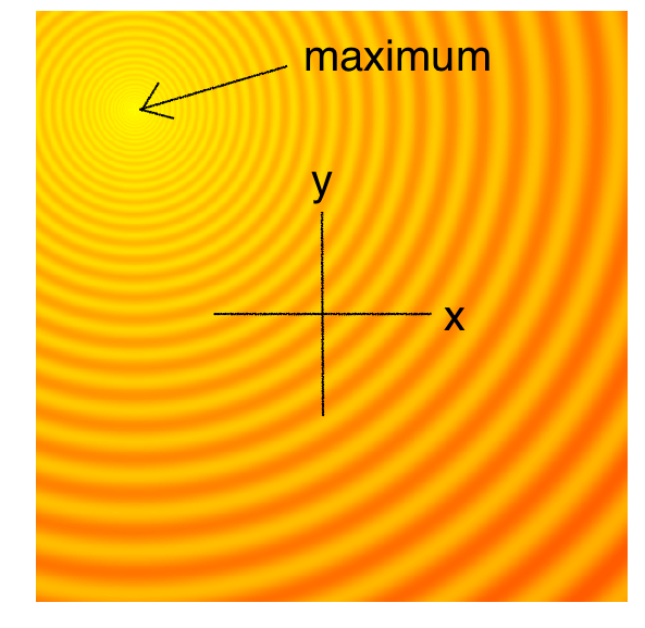
|
Rastrigin-2D Function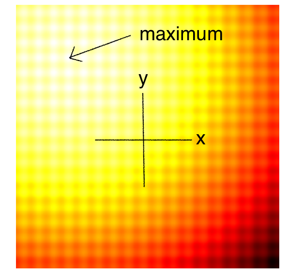
|
Although there are many definitions of evolution strategies, we can define an evolution strategy as an algorithm that provides the user a set of candidate solutions to evaluate a problem. The evaluation is based on an objective function that takes a given solution and returns a single fitness value. Based on the fitness results of the current solutions, the algorithm will then produce the next generation of candidate solutions that is more likely to produce even better results than the current generation. The iterative process will stop once the best known solution is satisfactory for the user.
Given an evolution strategy algorithm called EvolutionStrategy, we can use in the following way:
solver = EvolutionStrategy()
while True:
# ask the ES to give us a set of candidate solutions
solutions = solver.ask()
# create an array to hold the fitness results.
fitness_list = np.zeros(solver.popsize)
# evaluate the fitness for each given solution.
for i in range(solver.popsize):
fitness_list[i] = evaluate(solutions[i])
# give list of fitness results back to ES
solver.tell(fitness_list)
# get best parameter, fitness from ES
best_solution, best_fitness = solver.result()
if best_fitness > MY_REQUIRED_FITNESS:
break
Although the size of the population is usually held constant for each generation, they don’t need to be. The ES can generate as many candidate solutions as we want, because the solutions produced by an ES are sampled from a distribution whose parameters are being updated by the ES at each generation. I will explain this sampling process with an example of a simple evolution strategy.
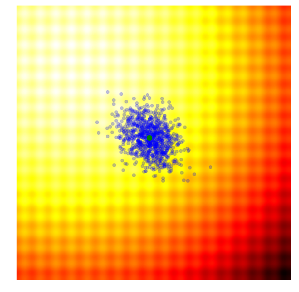
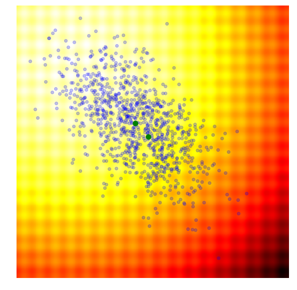
One of the simplest evolution strategy we can imagine will just sample a set of solutions from a Normal distribution, with a mean and a fixed standard deviation . In our 2D problem, and . Initially, is set at the origin. After the fitness results are evaluated, we set to the best solution in the population, and sample the next generation of solutions around this new mean. This is how the algorithm behaves over 20 generations on the two problems mentioned earlier:
|

|
In the visualisation above, the green dot indicates the mean of the distribution at each generation, the blue dots are the sampled solutions, and the red dot is the best solution found so far by our algorithm.
This simple algorithm will generally only work for simple problems. Given its greedy nature, it throws away all but the best solution, and can be prone to be stuck at a local optimum for more complicated problems. It would be beneficial to sample the next generation from a probability distribution that represents a more diverse set of ideas, rather than just from the best solution from the current generation.
One of the oldest black-box optimisation algorithms is the genetic algorithm. There are many variations with many degrees of sophistication, but I will illustrate the simplest version here.
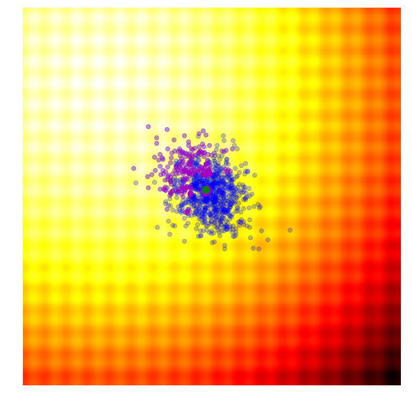
The idea is quite simple: keep only 10% of the best performing solutions in the current generation, and let the rest of the population die. In the next generation, to sample a new solution is to randomly select two solutions from the survivors of the previous generation, and recombine their parameters to form a new solution. This crossover recombination process uses a coin toss to determine which parent to take each parameter from. In the case of our 2D toy function, our new solution might inherit or from either parents with 50% chance. Gaussian noise with a fixed standard deviation will also be injected into each new solution after this recombination process.

|
|
The figure above illustrates how the simple genetic algorithm works. The green dots represent members of the elite population from the previous generation, the blue dots are the offsprings to form the set of candidate solutions, and the red dot is the best solution.
Genetic algorithms help diversity by keeping track of a diverse set of candidate solutions to reproduce the next generation. However, in practice, most of the solutions in the elite surviving population tend to converge to a local optimum over time. There are more sophisticated variations of GA out there, such as CoSyNe, ESP, and NEAT, where the idea is to cluster similar solutions in the population together into different species, to maintain better diversity over time.
A shortcoming of both the Simple ES and Simple GA is that our standard deviation noise parameter is fixed. There are times when we want to explore more and increase the standard deviation of our search space, and there are times when we are confident we are close to a good optima and just want to fine tune the solution. We basically want our search process to behave like this:

|
|
Amazing isn’it it? The search process shown in the figure above is produced by Covariance-Matrix Adaptation Evolution Strategy (CMA-ES). CMA-ES an algorithm that can take the results of each generation, and adaptively increase or decrease the search space for the next generation. It will not only adapt for the mean and sigma parameters, but will calculate the entire covariance matrix of the parameter space. At each generation, CMA-ES provides the parameters of a multi-variate normal distribution to sample solutions from. So how does it know how to increase or decrease the search space?
Before we discuss its methodology, let’s review how to estimate a covariance matrix. This will be important to understand CMA-ES’s methodology later on. If we want to estimate the covariance matrix of our entire sampled population of size of , we can do so using the set of equations below to calculate the maximum likelihood estimate of a covariance matrix . We first calculate the means of each of the and in our population:
The terms of the 2×2 covariance matrix will be:
Of course, these resulting mean estimates and , and covariance terms , , will just be an estimate to the actual covariance matrix that we originally sampled from, and not particularly useful to us.
CMA-ES modifies the above covariance calculation formula in a clever way to make it adapt well to an optimisation problem. I will go over how it does this step-by-step. Firstly, it focuses on the best solutions in the current generation. For simplicity let’s set to be the best 25% of solutions. After sorting the solutions based on fitness, we calculate the mean of the next generation as the average of only the best 25% of the solutions in current population , i.e.:
Next, we use only the best 25% of the solutions to estimate the covariance matrix of the next generation, but the clever hack here is that it uses the current generation’s , rather than the updated parameters that we had just calculated, in the calculation:
Armed with a set of , , , , and parameters for the next generation , we can now sample the next generation of candidate solutions.
Below is a set of figures to visually illustrate how it uses the results from the current generation to construct the solutions in the next generation :
 Step 1 Step 1 |
 Step 2 Step 2 |
 Step 3 Step 3 |
 Step 4 Step 4 |
Let’s visualise the scheme one more time, on the entire search process on both problems:
|
|
Because CMA-ES can adapt both its mean and covariance matrix using information from the best solutions, it can decide to cast a wider net when the best solutions are far away, or narrow the search space when the best solutions are close by. My description of the CMA-ES algorithm for a 2D toy problem is highly simplified to get the idea across. For more details, I suggest reading the CMA-ES Tutorial prepared by Nikolaus Hansen, the author of CMA-ES.
This algorithm is one of the most popular gradient-free optimisation algorithms out there, and has been the algorithm of choice for many researchers and practitioners alike. The only real drawback is the performance if the number of model parameters we need to solve for is large, as the covariance calculation is , although recently there has been approximations to make it . CMA-ES is my algorithm of choice when the search space is less than a thousand parameters. I found it still usable up to ~ 10K parameters if I’m willing to be patient.
Imagine if you had built an artificial life simulator, and you sample a different neural network to control the behavior of each ant inside an ant colony. Using the Simple Evolution Strategy for this task will optimise for traits and behaviours that benefit individual ants, and with each successive generation, our population will be full of alpha ants who only care about their own well-being.
Instead of using a rule that is based on the survival of the fittest ants, what if you take an alternative approach where you take the sum of all fitness values of the entire ant population, and optimise for this sum instead to maximise the well-being of the entire ant population over successive generations? Well, you would end up creating a Marxist utopia.
A perceived weakness of the algorithms mentioned so far is that they discard the majority of the solutions and only keep the best solutions. Weak solutions contain information about what not to do, and this is valuable information to calculate a better estimate for the next generation.
Many people who studied RL are familiar with the REINFORCE paper. In this 1992 paper, Williams outlined an approach to estimate the gradient of the expected rewards with respect to the model parameters of a policy neural network. This paper also proposed using REINFORCE as an Evolution Strategy, in Section 6 of the paper. This special case of REINFORCE-ES was expanded later on in Parameter-Exploring Policy Gradients (PEPG, 2009) and Natural Evolution Strategies (NES, 2014).
In this approach, we want to use all of the information from each member of the population, good or bad, for estimating a gradient signal that can move the entire population to a better direction in the next generation. Since we are estimating a gradient, we can also use this gradient in a standard SGD update rule typically used for deep learning. We can even use this estimated gradient with Momentum SGD, RMSProp, or Adam if we want to.
The idea is to maximise the expected value of the fitness score of a sampled solution. If the expected result is good enough, then the best performing member within a sampled population will be even better, so optimising for the expectation might be a sensible approach. Maximising the expected fitness score of a sampled solution is almost the same as maximising the total fitness score of the entire population.
If is a solution vector sampled from a probability distribution function , we can define the expected value of the objective function as:
where are the parameters of the probability distribution function. For example, if is a normal distribution, then would be and . For our simple 2D toy problems, each ensemble is a 2D vector .
The NES paper contains a nice derivation of the gradient of with respect to . Using the same log-likelihood trick as in the REINFORCE algorithm allows us to calculate the gradient of :
In a population size of , where we have solutions , , , we can estimate this gradient as a summation:
With this gradient , we can use a learning rate parameter (such as 0.01) and start optimising the parameters of pdf so that our sampled solutions will likely get higher fitness scores on the objective function . Using SGD (or Adam), we can update for the next generation:
and sample a new set of candidate solutions from this updated pdf, and continue until we arrive at a satisfactory solution.
In Section 6 of the REINFORCE paper, Williams derived closed-form formulas of the gradient , for the special case where is a factored multi-variate normal distribution (i.e., the correlation parameters are zero). In this special case, are the and vectors. Therefore, each element of a solution can be sampled from a univariate normal distribution .
The closed-form formulas for , for each individual element of vector on each solution in the population can be derived as:
For clarity, I use the index of , to count across parameter space, and this is not to be confused with superscript , used to count across each sampled member of the population. For our 2D problems, , , , , , in this context.
These two formulas can be plugged back into the approximate gradient formula to derive explicit update rules for and . In the papers mentioned above, they derived more explicit update rules, incorporated a baseline, and introduced other tricks such as antithetic sampling in PEPG, which is what my implementation is based on. NES proposed incorporating the inverse of the Fisher Information Matrix into the gradient update rule. But the concept is basically the same as other ES algorithms, where we update the mean and standard deviation of a multi-variate normal distribution at each new generation, and sample a new set of solutions from the updated distribution. Below is a visualization of this algorithm in action, following the formulas described above:

|
|
We see that this algorithm is able to dynamically change the ’s to explore or fine tune the solution space as needed. Unlike CMA-ES, there is no correlation structure in our implementation, so we don’t get the diagonal ellipse samples, only the vertical or horizontal ones, although in principle we can derive update rules to incorporate the entire covariance matrix if we needed to, at the expense of computational efficiency.
I like this algorithm because like CMA-ES, the ’s can adapt so our search space can be expanded or narrowed over time. Because the correlation parameter is not used in this implementation, the efficiency of the algorithm is so I use PEPG if the performance of CMA-ES becomes an issue. I usually use PEPG when the number of model parameters exceed several thousand.
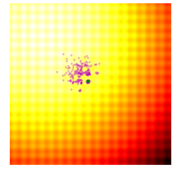
In OpenAI’s paper, they implement an evolution strategy that is a special case of the REINFORCE-ES algorithm outlined earlier. In particular, is fixed to a constant number, and only the parameter is updated at each generation. Below is how this strategy looks like, with a constant parameter:
|

|
In addition to the simplification, this paper also proposed a modification of the update rule that is suitable for parallel computation across different worker machines. In their update rule, a large grid of random numbers have been pre-computed using a fixed seed. By doing this, each worker can reproduce the parameters of every other worker over time, and each worker needs only to communicate a single number, the final fitness result, to all of the other workers. This is important if we want to scale evolution strategies to thousands or even a million workers located on different machines, since while it may not be feasible to transmit an entire solution vector a million times at each generation update, it may be feasible to transmit only the final fitness results. In the paper, they showed that by using 1440 workers on Amazon EC2 they were able to solve the Mujoco Humanoid walking task in ~ 10 minutes.
I think in principle, this parallel update rule should work with the original algorithm where they can also adapt , but perhaps in practice, they wanted to keep the number of moving parts to a minimum for large-scale parallel computing experiments. This inspiring paper also discussed many other practical aspects of deploying ES for RL-style tasks, and I highly recommend going through it to learn more.
Most of the algorithms above are usually combined with a fitness shaping method, such as the rank-based fitness shaping method I will discuss here. Fitness shaping allows us to avoid outliers in the population from dominating the approximate gradient calculation mentioned earlier:
If a particular is much larger than other in the population, then the gradient might become dominated by this outliers and increase the chance of the algorithm being stuck in a local optimum. To mitigate this, one can apply a rank transformation of the fitness. Rather than use the actual fitness function, we would rank the results and use an augmented fitness function which is proportional to the solution’s rank in the population. Below is a comparison of what the original set of fitness may look like, and what the ranked fitness looks like:

What this means is supposed we have a population size of 101. We would evaluate each population to the actual fitness function, and then sort the solutions based by their fitness. We will assign an augmented fitness value of -0.50 to the worse performer, -0.49 to the second worse solution, …, 0.49 to the second best solution, and finally a fitness value of 0.50 to the best solution. This augmented set of fitness values will be used to calculate the gradient update, instead of the actual fitness values. In a way, it is a similar to just applying Batch Normalization to the results, but more direct. There are alternative methods for fitness shaping but they all basically give similar results in the end.
I find fitness shaping to be very useful for RL tasks if the objective function is non-deterministic for a given policy network, which is often the cases on RL environments where maps are randomly generated and various opponents have random policies. It is less useful for optimising for well-behaved functions that are deterministic, and the use of fitness shaping can sometimes slow down the time it takes to find a good solution.
Although ES might be a way to search for more novel solutions that are difficult for gradient-based methods to find, it still vastly underperforms gradient-based methods on many problems where we can calculate high quality gradients. For instance, only an idiot would attempt to use a genetic algorithm for image classification. But sometimes such people do exist in the world, and sometimes these explorations can be fruitful!
Since all ML algorithms should be tested on MNIST, I also tried to apply these various ES algorithms to find weights for a small, simple 2-layer convnet used to classify MNIST, just to see where we stand compared to SGD. The convnet only has ~ 11k parameters so we can accommodate the slower CMA-ES algorithm. The code and the experiments are available here.
<!–
______
class Net(nn.Module):
def __init__(self):
super(Net, self).__init__()
self.num_filter1 = 8
self.num_filter2 = 16
self.num_padding = 2
self.filter_size = 5
# input is 28x28
self.conv1 = nn.Conv2d(1,
self.num_filter1,
self.filter_size,
padding=self.num_padding)
# feature map size is 14*14 by pooling
self.conv2 = nn.Conv2d(self.num_filter1,
self.num_filter2,
self.filter_size,
padding=self.num_padding)
# feature map size is 7*7 by pooling
self.fc = nn.Linear(self.num_filter2*7*7, 10)
def forward(self, x):
x = F.max_pool2d(F.relu(self.conv1(x)), 2)
x = F.max_pool2d(F.relu(self.conv2(x)), 2)
x = x.view(-1, self.num_filter2*7*7)
x = self.fc(x)
return F.log_softmax(x)
______
–>
Below are the results for various ES methods, using a population size of 101, over 300 epochs. We keep track of the model parameters that performed best on the entire training set at the end of each epoch, and evaluate this model once on the test set after 300 epochs. It is interesting how sometimes the test set’s accuracy is higher than the training set for the models that have lower scores.
| Method | Train Set | Test Set |
|---|---|---|
| Adam (BackProp) Baseline | 99.8 | 98.9 |
| Simple GA | 82.1 | 82.4 |
| CMA-ES | 98.4 | 98.1 |
| OpenAI-ES | 96.0 | 96.2 |
| PEPG | 98.5 | 98.0 |

We should take these results with a grain of salt, since they are based on a single run, rather than the average of 5-10 runs. The results based on a single-run seem to indicate that CMA-ES is the best at the MNIST task, but the PEPG algorithm is not that far off. Both of these algorithms achieved ~ 98% test accuracy, 1% lower than the SGD/ADAM baseline. Perhaps the ability to dynamically alter its covariance matrix, and standard deviation parameters over each generation allowed it to fine-tune its weights better than OpenAI’s simpler variation.
There are probably open source implementations of all of the algorithms described in this article. The author of CMA-ES, Nikolaus Hansen, has been maintaining a numpy-based implementation of CMA-ES with lots of bells and whistles. His python implementation introduced me to the training loop interface described earlier. Since this interface is quite easy to use, I also implemented the other algorithms such as Simple Genetic Algorithm, PEPG, and OpenAI’s ES using the same interface, and put it in a small python file called es.py, and also wrapped the original CMA-ES library in this small library. This way, I can quickly compare different ES algorithms by just changing one line:
import es
#solver = es.SimpleGA(...)
#solver = es.PEPG(...)
#solver = es.OpenES(...)
solver = es.CMAES(...)
while True:
solutions = solver.ask()
fitness_list = np.zeros(solver.popsize)
for i in range(solver.popsize):
fitness_list[i] = evaluate(solutions[i])
solver.tell(fitness_list)
result = solver.result()
if result[1] > MY_REQUIRED_FITNESS:
break
You can look at es.py on GitHub and the IPython notebook examples using the various ES algorithms.
In this IPython notebook that accompanies es.py, I show how to use the ES solvers in es.py to solve a 100-Dimensional version of the Rastrigin function with even more local optimum points. The 100-D version is somewhat more challenging than the trivial 2D version used to produce the visualizations in this article. Below is a comparison of the performance for various algorithms discussed:

On this 100-D Rastrigin problem, none of the optimisers got to the global optimum solution, although CMA-ES comes close. CMA-ES blows everything else away. PEPG is in 2nd place, and OpenAI-ES / Genetic Algorithm falls behind. I had to use an annealing schedule to gradually lower for OpenAI-ES to make it perform better for this task.

Final solution that CMA-ES discovered for 100-D Rastrigin function.
Global optimal solution is a 100-dimensional vector of exactly 10.
so proud of my little dude … pic.twitter.com/j5j61vQxP0
— hardmaru (@hardmaru) July 23, 2017
In the next article, I will look at applying ES to other experiments and more interesting problems. Please check it out!
If you find this work useful, please cite it as:
@article{ha2017visual,

  title   = "A Visual Guide to Evolution Strategies",

  author  = "Ha, David",

  journal = "blog.otoro.net",

  year    = "2017",

  url     = "https://blog.otoro.net/2017/10/29/visual-evolution-strategies/"

}
Below are a few links to information related to evolutionary computing which I found useful or inspiring.
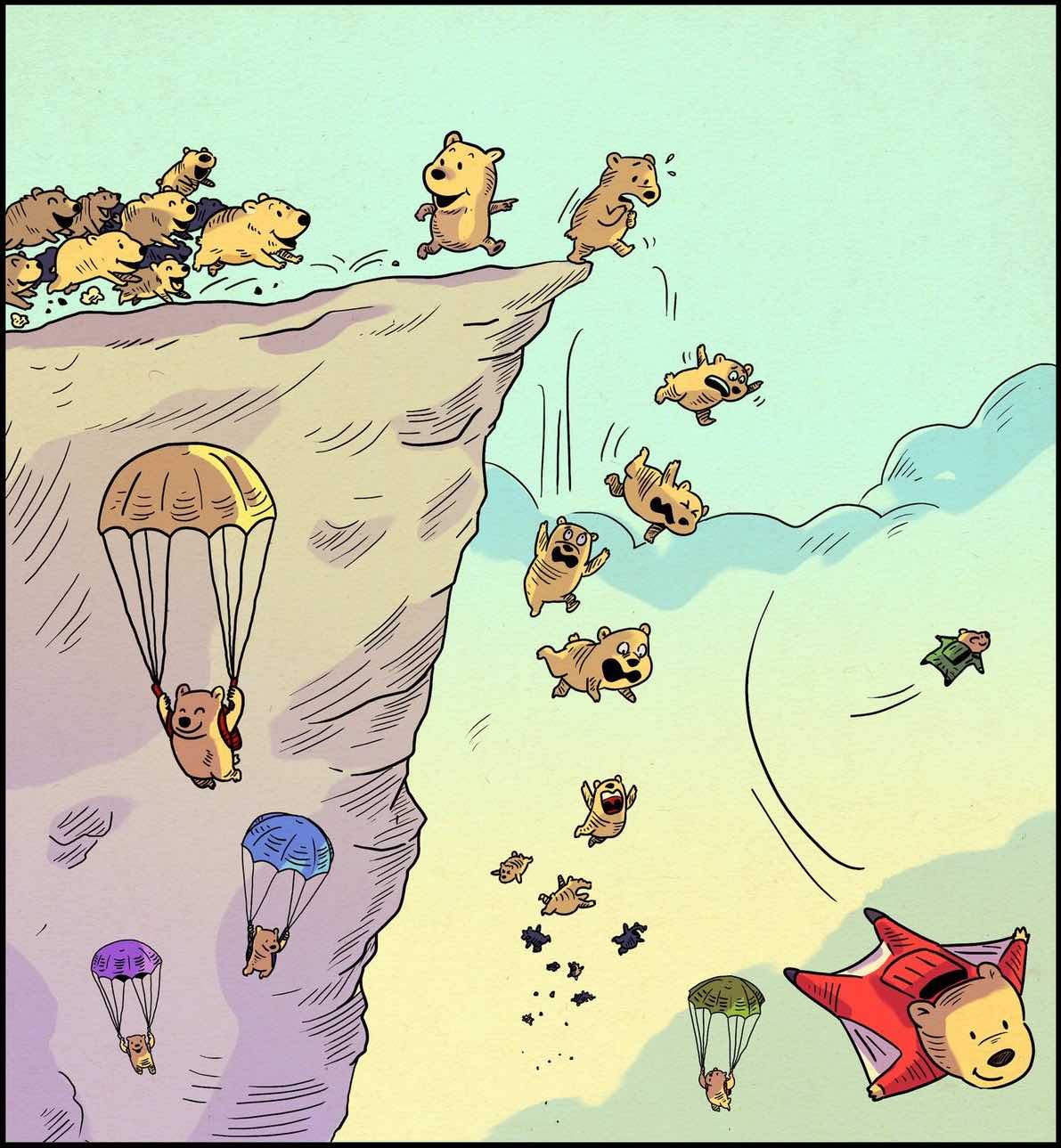
Image Credits of Lemmings Jumping off a Cliff. Your results may vary when investing in ICOs.
CMA-ES: Official Reference Implementation on GitHub, Tutorial, Original CMA-ES Paper from 2001, Overview Slides
Simple Statistical Gradient-Following Algorithms for Connectionist Reinforcement Learning (REINFORCE), 1992.
Parameter-Exploring Policy Gradients, 2009.
Natural Evolution Strategies, 2014.
Evolution Strategies as a Scalable Alternative to Reinforcement Learning, OpenAI, 2017.
Risto Miikkulainen’s Slides on Neuroevolution.
A Neuroevolution Approach to General Atari Game Playing, 2013.
Kenneth Stanley’s Talk on Why Greatness Cannot Be Planned: The Myth of the Objective, 2015.
Neuroevolution: A Different Kind of Deep Learning. The quest to evolve neural networks through evolutionary algorithms.
Compressed Network Search Finds Complex Neural Controllers with a Million Weights.
Karl Sims Evolved Virtual Creatures, 1994.
Evolved Step Climbing Creatures.
Super Mario World Agent Mario I/O, Mario Kart 64 Controller using using NEAT Algorithm.
Ingo Rechenberg, the inventor of Evolution Strategies.
A Tutorial on Differential Evolution with Python.
PathNet: Evolution Channels Gradient Descent in Super Neural Networks
Neural Network Evolution Playground with Backprop NEAT
Evolved Neural Art Gallery using CPPN Implementation
Evolution of Inverted Double Pendulum Swing Up Controller
I’ve never worked in the field of computer vision and has no idea how the magic could work when an autonomous car is configured to tell apart a stop sign from a pedestrian in a red hat. To motivate myself to look into the maths behind object rec…
We’ve developed a hierarchical reinforcement learning algorithm that learns high-level actions useful for solving a range of tasks, allowing fast solving of tasks requiring thousands of timesteps. Our algorithm, when applied to a set of navigation prob…
Our latest robotics techniques allow robot controllers, trained entirely in simulation and deployed on physical robots, to react to unplanned changes in the environment as they solve simple tasks. That is, we’ve used these techniques to build closed-lo…
 –>
–>