LSTM: Why It Was Born, How It Fixes RNN, and Why It Changed Sequence Learning

Sequence data is messy. Words depend on earlier words, notes depend on earlier notes, signals depend on earlier signals, and the past has this annoying habit of refusing to stay irrelevant. That is exactly why recurrent models exist in the first place.

But vanilla RNNs break in a very specific way. They are built for memory, yet they are bad at remembering. That contradiction is the entire reason LSTM exists.

1. Why RNN Was Not Enough

The goal of an RNN was straightforward: handle sequential data where previous information matters.

Common examples include:

• language modeling
• speech recognition
• time series forecasting
• translation
• chat-like sequence prediction

In theory, an RNN should remember all previous information.

Consider this sentence:

“The boy who lives next door is tall.”

To predict “is tall”, the model must remember “boy”, which appeared many words earlier.

That is the core job of a sequence model. RNN should do it.

But in practice, it fails.

2. Where RNN Fails: The Real Problem

The fundamental issue with a vanilla RNN is simple:

It cannot remember long-term dependencies.

Why this matters

Imagine reading:

“I grew up in France… so I speak fluent ______.”

You instantly know the answer is French.

Why? Because your brain keeps track of information from far back in the sentence.

RNN is supposed to do the same thing.

3. How RNN Should Work

At first glance, RNN seems perfect for sequence data:

• it reads words one by one
• it keeps a hidden state as memory
• it passes that memory forward through the sequence

So theoretically:

RNN should remember everything from the past.

That is the promise.

The problem is that the promise collapses under training.

4. What Actually Happens: The Failure

During training, RNNs use Backpropagation Through Time (BPTT).

That means:

• errors flow backward through each time step
• gradients are multiplied again and again across the sequence

And here is the real problem:

Gradients shrink exponentially over time.

Mathematically, the gradient through time behaves like a repeated product:

In the simplified case:

• if values are less than 1, gradients shrink → vanish
• if values are greater than 1, gradients grow → explode

Think of it like this:

• recent words have strong influence
• old words have almost zero influence

Why?

Because activation functions like sigmoid and tanh produce small derivatives, and repeated multiplication makes the gradient nearly zero.

Example:

So the signal from earlier words dies before it reaches the output.

That is why the model becomes biased toward the most recent inputs.

6. What This Means in Practice

A vanilla RNN behaves like someone with short-term memory only:

• it remembers the last few words
• it forgets important context from earlier

So in the sentence:

“I grew up in France… so I speak fluent ______.”

the model may remember “so I speak fluent” but forget “France”.

That may leads to the wrong prediction.

7. The Core Problem, Stated Clearly

RNN cannot learn long-term dependencies because gradients vanish over time.

That is the vanishing gradient problem.

Because of this:

• RNN focuses mostly on recent inputs
• long-range relationships are lost
• early tokens contribute almost nothing to learning

This is why RNNs work reasonably well for short sequences, but begin to break down on longer ones.

8. Why Exactly This Happens

There are two main reasons:

1. activation functions like tanh and sigmoid compress values into small ranges
2. repeated multiplication through many time steps reduces the gradient toward zero

So early time steps receive almost no learning signal.

That is why:

• recent tokens affect the output more
• distant tokens barely matter

9. The Real Question Researchers Asked

Researchers asked something much better than “how do we make an RNN slightly less terrible?”

They asked:

Can we build a neural network that remembers important information for a long time and forgets useless information?

That question matters because human memory works that way.

We remember:

• important facts
• key events

But forget:

• noise
• irrelevant details

That insight led to Long Short-Term Memory (LSTM).

10. The Turning Point

Researchers realized:

The real problem was not sequence modeling itself.
The real problem was memory retention.

So the question changed from:

“Can we process sequences?”

to:

“Can we build a network that decides what to remember and what to forget?”

That question directly led to LSTM.

11. Birth of LSTM (1997)

Key paper

Hochreiter, S., & Schmidhuber, J. (1997). Long Short-Term Memory. Neural Computation, 9(8), 1735–1780.

Core idea

Instead of letting gradients vanish, force constant error flow.

That is the entire point of the architecture.

How LSTM Fixed Memory: The Real Innovation

12. The Basic Idea of LSTM

LSTM separates memory into two ideas:

• Short Term Context (STC)
• Long Term Context (LTC)

Key concept

• important information from STC → moves to LTC
• if something becomes not important later → removed from LTC

That is the core design philosophy.

13. The Key Idea of LSTM

LSTM introduces a new concept:

Memory Cell (Cell State)

Think of it as:

a conveyor belt running through time.

Information can travel through this cell almost unchanged.

This solves the gradient issue because:

• gradients flow through additive updates
• not repeated multiplications

So they do not vanish easily.

14. Problem with RNN

In RNN:

• there is only one path to maintain memory/state
• this path tries to store both STC and LTC

Reality:

• it is not possible to store both effectively in the same path
• STC dominates LTC
• result → long-term dependencies are lost

That is the core problem.

15. Solution Idea (LSTM)

LSTM introduces another path across timesteps.

This path specifically carries LTC (cell state).

Important information:

• stored early
• preserved till later timesteps
• unless explicitly removed

That is the innovation.

16. Enter LSTM: A Memory System, Not Just a Network

Instead of a single hidden state like an RNN, LSTM introduces something more powerful:

A Cell State (Long-Term Memory)

Think of it like a highway running through time.

• information flows almost unchanged
• memory can persist across long sequences
• stable memory is easier to maintain

This is the central structural advantage.

17. The Highway Analogy

Imagine:

• RNN = narrow road → information gets lost
• LSTM = highway → information flows smoothly

But here is the twist:

Not everything should stay on the highway.

So LSTM adds control systems.

18. Two Types of Memory

LSTM has two kinds of memory:

• Long Term Memory → Cell State (Cₜ)
• Short Term Memory → Hidden State (hₜ)

This distinction matters.

• the cell state stores memory across time
• the hidden state exposes what is needed now

19. Interaction at Time (t)

Inputs:

• previous cell state → (Cₜ₋₁)
• previous hidden state → (hₜ₋₁)
• current input → (xₜ)

Outputs:

• current cell state → (Cₜ)
• current hidden state → (hₜ)

So, each timestep is not just “output and move on”; it is a controlled memory update.

20. Main Operations

At each timestep, LSTM does two main things:

1. Update the cell state:
   Cₜ₋₁ → Cₜ
2. Compute the hidden state:
   hₜ

That is the entire recurrent step, but with memory control built in.

21. Decision Logic

Based on current input (xₜ), LSTM decides:

• what to remove from long-term memory
• what to add to long-term memory

This is why it works better than a vanilla RNN, which blindly keeps pushing memory forward.

22. The Secret Weapon: Gates

LSTM introduced gates.

These are small decision makers that ask:

“Should I allow this information or not?”

They output values between 0 and 1:

• 0 → block completely
• 1 → allow fully
• values in between → partial flow

Three gates exist:

1. Forget Gate
2. Input Gate
3. Output Gate

These gates act like decision systems.

23. The Three Gates That Control Memory

Forget Gate

Question it answers:

What should we forget from the past?

Input Gate

Question it answers:

What new information should be stored?

Output Gate

Question it answers:

What part of memory should influence the output?

Together, these gates define the LSTM.

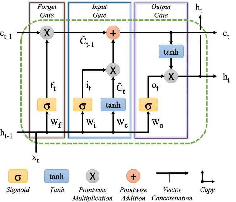
Detailed LSTM Architecture

24. Forget Gate

Purpose

• Remove unnecessary info from the cell state.

Computation

Input:

• hₜ₋₁
• xₜ

Concatenate:

• [hₜ₋₁, xₜ]

Then:

• fₜ = σ( [hₜ₋₁, xₜ]W_f + b_f )

Dimensions example

If:

• (xₜ) is 4-dimensional
• hidden state has 3 unit

Then concatenated input has dimension:

• 4 + 3 = 7

So:

• Weight matrix → (7 × 3)
• Bias → (3)
• Output (fₜ) → (1 × 3)

Cell update for the forget part

• Cₜ₋₁ ⊙ fₜ

Because fₜ ∈ (0,1), each dimension of Cₜ₋₁ is scaled individually:

• if fₜ ≈ 1 → keep
• if fₜ ≈ 0 → forget
• otherwise → partially reduce

Interpretation

The forget gate controls:

“How much of each memory dimension should pass?”

The decision is based on:

• Current input: xₜ
• Previous hidden state: hₜ₋₁

25. Input Gate

Purpose

• Add new important information to the cell state.

Computation

Gate decision:

• iₜ = σ( [hₜ₋₁, xₜ] W_i + b_i )

Candidate memory:

• C̃ₜ = tanh( [hₜ₋₁, xₜ] W_c + b_c )

Dimensions example

• [hₜ₋₁, xₜ] → (1 × 7)
• W_i → (7 × 3)
• b_i → (1 × 3)
• iₜ → (1 × 3)
• C̃ₜ → (1 × 3)

Interpretation

• Candidate = “what can be added”
• Input gate = “what should actually be added”

Meaning

The input gate controls how much of (C̃ₜ) is added.

So:

• candidate cell state = potential information
• input gate = filter deciding what enters the memory

26. Cell State Update

Now the key update step:

• Cₜ = (Cₜ₋₁ ⊙ fₜ) + (iₜ ⊙ C̃ₜ)

Breakdown

1. First term: Cₜ₋₁ ⊙ fₜ

• Old memory is filtered. This means some useless data is forgotten.

2. Second term: iₜ ⊙ C̃ₜ

• New useful information is added. This is the current input, filtered by relevance.

Dimensions

• Cₜ → (1 × 3)

Why this matters

This additive update is the key reason gradients survive longer.

Instead of repeatedly multiplying and shrinking signal strength, LSTM adds information to a stable memory path.

27. Why LSTM Works Mathematically (Full Derivation)

From the cell update:

• Cₜ = fₜ ⊙ Cₜ₋₁ + iₜ ⊙ C̃ₜ

In the simplified derivation, the direct path from Cₜ₋₁ to Cₜ is controlled by fₜ, so:

This means:

• if fₜ ≈ 1, memory and gradients are preserved
• if fₜ ≈ 0, memory is forgotten

Extending Across Time

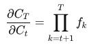
So the cell state provides a stable, controlled path for long-term information.

By contrast, in RNN:

and each factor includes repeated matrix multiplication and activation derivatives, which often shrink toward zero.

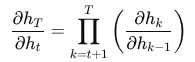
Gradient Flow through hidden state:

• hₜ = oₜ ⊙ tanh(Cₜ)

So:

• ∂hₜ / ∂Cₜ = oₜ ⊙ (1 − tanh²(Cₜ))

This is why the output is bounded and why gradients remain more stable.

So LSTM separates gradient flow into two paths:

• a nonlinear exposed path through hₜ
• a stable memory path through Cₜ

28. Key Insight: Vanishing Gradient Problem

— In RNN:

• vanishing gradients cause information loss at each step
• long timesteps become disastrous

— In LSTM:

• possible to have very small information loss
• because the cell state supports stable propagation

Important notes:

For longer timesteps, the information loss is negligible.

Special cases

— Case 1

If:

• fₜ = 1

Then:

• Cₜ = Cₜ₋₁ + iₜ ⊙ C̃ₜ

Meaning: no information lost

— Case 2

If:

• iₜ = 0

Then:

• Cₜ = Cₜ₋₁ ⊙ fₜ

Meaning: no new information added

This is exactly the kind of controllable memory behavior RNN lacks.

29. Long Sequence Insight

LSTM can preserve long-term context from start to end.

That makes it useful for:

• long sentences
• delayed dependencies
• sequences where early tokens matter much later

This is one of the most important conceptual advantages of the architecture.

30. Output Gate

Computation

• oₜ = σ( [hₜ₋₁, xₜ] W_o + b_o )

Dimensions example

• [hₜ₋₁, xₜ] → (1 × 7)
• W_o → (7 × 3)
• b_o → (1 × 3)
• oₜ → (1 × 3)

Hidden state

• hₜ = oₜ ⊙ tanh(Cₜ)

What this does

1. Apply tanh to Cₜ → values in (-1, 1)
2. Apply filtering using oₜ

Interpretation

The output gate decides:

“Value for current hidden state (hₜ)”

This becomes the output passed to the next timestep.

Why Apply (tanh) Before the Output Gate Multiplies?

Why not directly use: hₜ = oₜ ⊙ Cₜ

31. Hidden State in LSTM

The hidden state in LSTM is:

• hₜ = oₜ ⊙ tanh(Cₜ)

Short answer

We apply tanh to control scale and stabilize the output. Otherwise, the hidden state can explode and training becomes unstable.

Deep intuition

What is (Cₜ)?

• it is the cell state
• it keeps accumulating information over time

Important point:

(Cₜ) is unbounded and can grow very large.

That is fine for memory storage, but terrible for direct exposure as output.

Problem if you use (Cₜ) directly

If you do: hₜ = oₜ ⊙ Cₜ

Then:

• if (Cₜ = 50), the output becomes huge
• if (Cₜ= -100), the output becomes extreme
• this propagates forward and makes the network unstable

That leads to:

• exploding activations
• unstable gradients
• poor training

Why tanh(Cₜ)?

Because tanh does this:

tanh(x) ∈ (-1, 1)

So no matter how large (Cₜ) gets:

the output is always controlled

Intuition

Think of it like this:

• Cₜ = raw memory (can be messy, large, and unfiltered)
• tanh = compress and normalize memory
• oₜ = decide what to show

So the actual flow is:

1. memory stored → ( Cₜ )
2. normalize → ( tanh(Cₜ) )
3. filter → multiply with ( oₜ )

Why not let the output gate handle everything?

The sigmoid output gate ( oₜ ) only scales from 0 to 1.

It cannot normalize large values.

Example:

• (Cₜ = 100)
• (oₜ = 0.9)

Then: hₜ = 0.9 · 100 = 90
That is still huge.

So:

• gate controls how much
• tanh controls how big

They do different jobs.

(tanh) ensures the hidden state remains bounded, while the output gate decides how much of that bounded information to expose.

Analogy

Think of ( Cₜ ) as raw water pressure in a pipe.
( tanh ) acts like a regulator that keeps pressure safe.
The output gate is the tap deciding how much water to release.

Final insight

This also helps with:

• smoother gradients
• better generalization
• stable training over long sequences

Putting It All Together

32. Summary of Flow

At each timestep:

— Forget gate

• removes irrelevant past info

— Input gate

• adds new important info

— Cell state update

• combines old filtered memory with new filtered information

— Output gate

• produces hidden state

33. Full LSTM Flow

Step by step:

1. Candidate state
   C̃ₜ = tanh( [hₜ₋₁, xₜ] W_c + b_c )
2. Input gate
   iₜ = σ( [hₜ₋₁, xₜ] W_i + b_i )
3. Forget gate
   fₜ = σ( [hₜ₋₁, xₜ] W_f + b_f )
4. Cell update
   Cₜ = ( Cₜ₋₁ ⊙ fₜ ) + ( iₜ ⊙ C̃ₜ )
5. Output gate
   oₜ = σ( [hₜ₋₁, xₜ] W_o + b_o )
6. Hidden state
   hₜ = oₜ ⊙ tanh(Cₜ)

34. Dimensional Summary

Component                | Shape
-------------------------|----------
xₜ                        | (1 × 4)
hₜ₋₁                      | (1 × 3)
Concat [hₜ₋₁, xₜ]          | (1 × 7)
Weights (W)              | (7 × 3)
Outputs (gates/cand.)    | (1 × 3)

35. LSTM Diagram Explained Step-by-Step

------------------------------------>
        Cell State (C_t)

👉 This is the Cell State (memory highway)

36. Step 1: Forget Gate

It takes two inputs:

• previous hidden state (hₜ₋₁)
• current input (xₜ)

h(t-1) ----\
             > [Forget Gate] ---> (multiplies with C(t-1))
x(t)  ------/

What it means

The forget gate decides what past information should be removed from memory.

It produces a value between 0 and 1, and multiplies it with the previous memory:

• Cₜ₋₁ ⊙ fₜ

So:

• 0 means forget completely
• 1 means keep completely

36. Step 2: Input Gate

This part has two pieces:

1. Input Gate using sigmoid
2. Candidate Memory using tanh

h(t-1), x(t) → [Input Gate]
h(t-1), x(t) → [Candidate Values]

Then they are combined.

What it means

The input gate decides what new information should be added.

So:

• Candidate (C̃ₜ) = possible new memory
• Gate (iₜ) = how much of it to allow

The result is:

iₜ ⊙ C̃ₜ

37. Step 3: Update Cell State

Now combine the old memory and the new memory.

This is the most important part of LSTM:

• Cₜ = (fₜ ⊙ Cₜ₋₁) + (iₜ ⊙ C̃ₜ)

Memory is updated by:

• removing old irrelevant information
• adding new useful information

This is why LSTM works:

• no repeated shrinking multiplication
• smooth information flow
• long-term memory stays alive

38. Step 4: Output Gate

h(t-1), x(t) → [Output Gate]  
C_t → tanh → × Output Gate → h(t)

What it means

The output gate decides what part of memory to use right now.

The final output is:

• hₜ = oₜ × tanh(Cₜ)

So, the cell state stores memory, and the output gate decides what gets exposed.

39. Final Full Diagram Logic

When you combine everything:

1. Left → forget old memory
2. Middle → add new memory, update cell state
3. Right → produce output

And the cell state flows straight across like a highway.

That horizontal path is the reason LSTM remembers long-term. The gates just control the traffic.

40. Super Simple Analogy

Think of LSTM like a smart notebook:

• ✂️ Forget Gate → erase useless notes
• ✍️ Input Gate → write important things
• 📖 Output Gate → read only what is needed

41. Intuition in One Line

RNN = “Try to remember everything” ❌
LSTM = “Remember smartly” ✅

42. Why LSTM Solves RNN Problems

Main innovations:

a. Memory Cell

Stores long-term information.

b. Gating Mechanism

Controls information flow.

c. Additive State Updates

Avoids exponential gradient decay.

d. Constant Error Flow

Gradients can propagate through many timesteps.

Because of this:

• LSTM can learn dependencies across hundreds or thousands of steps

43. Training Process

Steps

1. Forward pass through sequence
2. Compute loss
3. Backpropagation Through Time (BPTT)
4. Update weights using gradient descent

Complexity

• Time: O(T · n²)
• Memory: high, because all states must be stored

44. Improvements Over Time

LSTM did not remain the only gated recurrent design. Researchers pushed it further.

GRU (Cho et al., 2014)

• simpler version of LSTM
• fewer gates
• often faster and easier to train

Peephole LSTM

• gates can see the cell state
• adds extra access to memory information

Bidirectional LSTM

• uses past and future context
• useful when the full sequence is available

Attention Mechanism

• later reduced reliance on LSTM
• improved long-range dependency handling

45. Real Applications of LSTM

Before Transformers, LSTM dominated sequence learning.

Examples:

• Google Translate
• speech recognition
• handwriting recognition
• time series prediction
• NLP tasks like translation and chatbots
• stock prediction
• healthcare time series
• video processing

46. Limitations of LSTM

LSTM is powerful, but it is not magic.

It still has limits:

• slow training
• hard to parallelize
• memory intensive
• sequential computation
• difficulty with very long sequences
• replaced by Transformers in many tasks

47. Evolution After LSTM

Model progression:

RNN → LSTM → GRU → Attention → Transformers

Because even LSTM has limitations, which led to:

Attention is All You Need (Transformer).

48. Key Academic Sources

Here are referenced foundational and influential papers:

1. Hochreiter, S., & Schmidhuber, J. (1997). Long Short-Term Memory. Neural Computation, 9(8), 1735–1780.
2. Bengio, Y., Simard, P., & Frasconi, P. (1994). Learning long-term dependencies with gradient descent. IEEE Trans. Neural Networks.
3. Hochreiter, S. (1991). Untersuchungen zu dynamischen neuronalen Netzen.
4. Gers, F. A., Schmidhuber, J., & Cummins, F. (2000). Learning to forget: Continual prediction with LSTM. Neural Computation.
5. Graves, A. (2012). Supervised Sequence Labelling with RNNs.
6. Graves, A., Mohamed, A., & Hinton, G. (2013). Speech recognition with deep RNNs.
7. Cho, K. et al. (2014). Learning Phrase Representations using RNN Encoder–Decoder.
8. Greff, K. et al. (2017). LSTM: A Search Space Odyssey.
9. Olah, C. (2015). Understanding LSTM Networks.
10. Sak, H., Senior, A., & Beaufays, F. (2014). Long short-term memory recurrent neural network architectures for large scale acoustic modeling.

49. Finally

LSTM did not just improve RNN.
It changed the idea of memory in neural networks.

Instead of forcing the model to remember everything,
it taught the model how to remember.

RNN failed because gradients vanished over time, making it forget long-term dependencies.

LSTM was born to solve that by using a cell state and gates to control what to remember, what to forget, and what to use.

50. About the Author

Alok Ranjan Singh is a machine learning enthusiast and writer who enjoys breaking down deep learning ideas into clear, intuitive explanations. This article reflects an ongoing effort to study sequence models, gradient flow, and the mechanics behind memory in neural networks.

Connect with me on LinkedIn for discussions:
🔗 LinkedIn Profile Link

---

LSTM: Why It Was Born, How It Fixes RNN, and Why It Changed Sequence Learning was originally published in Towards AI on Medium, where people are continuing the conversation by highlighting and responding to this story.