What’s the problem?
Imagine a small business that uses an LLM to triage incoming sales leads. Lead A has an 80% chance of securing a modest $300 job. Lead B has a smaller 20% chance of leading to a much more profitable $1,400 job. Both options have equal expected value. The LLM is asked, “Which lead should we call first today?” and the model recommends A. But later, in a separate session, the model is asked, “How much should we be willing to sell each lead for?” and the model assigns B the higher value.
This was the pattern I observed in a 25,920-call experiment across four models: Claude Opus 4.7, DeepSeek V4-Pro, Google Gemini 3 Flash Preview, and OpenAI GPT-5.5. The design used 28 gamble pairs, eight dominance checks, three prompt formats, the lowest and highest reasoning settings for each model, and 10 samples per cell. The result was not just that independent judgments often disagreed even on the highest reasoning settings; the models also frequently chose the safer modest-payoff “P-bet” yet valued the riskier high-payoff “D-bet” more, the same type of inconsistency seen in the original human Lichtenstein-Slovic (L-S) preference-reversal studies of the 1970s.[1]
Here you can see the average choice-valuation inconsistency rates across the four models.
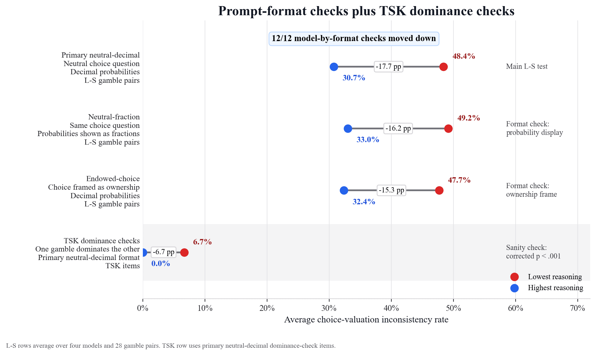
The first three rows show the inconsistency rates for the three prompt formats that were used: primary neutral-decimal format (probabilities shown as decimals), neutral-fraction format (probabilities shown as fractions in bullet form), and endowed-choice format (probabilities shown as decimals and framed in terms of ownership). In the primary format, inconsistency was common at the lowest reasoning settings, 48.4%, and lower, though still high, at 30.7% for the highest reasoning settings. The last row shows the inconsistency rate on the “TSK” dominance checks (where one gamble dominates the other, inspired by Tversky-Slovic-Kahneman[2]). This rate was low and suggests the main result is not due to a generic failure to compare all gambles, but instead appears in cases where probability and payoff pull in opposite directions.
How is the inconsistency rate defined?
Each L-S pair had a higher-probability/smaller-payoff P-bet and a lower-probability/larger-payoff D-bet, with some being near equal expected value (EV) and some being modestly P-EV-dominant or D-EV-dominant. For each model, reasoning setting, prompt format, and gamble pair, I made separate stateless (no memory) API calls for the direct choice question (which gamble the model prefers), P-bet valuation (the selling price the model assigns to the P-bet), and D-bet valuation (the selling price the model assigns to the D-bet).
For each cell


Let

Then the integrated inconsistency rate is:

The first term is the classic direction: choose P, price D higher. The second term is the opposite: choose D, price P higher.
For example, suppose eight of 10 choice samples pick P. Separately, the P-valuation and D-valuation samples imply that D is priced above P 60% of the time, P above D 30% of the time, and the remaining 10% are ties. Splitting ties evenly gives


If choice and valuation always implied the same ranking, the inconsistency rate would be 0; if they always implied opposite rankings, it would be 1.
I also report the lower bound:

This is the minimum disagreement forced by the observed choice and valuation margins, which can be seen in the figure below. If this bound is positive, even the most favorable possible pairing of choice and valuation answers cannot remove all disagreement.
Is the disagreement just random noise?
Independent samples can disagree merely because both procedures are stochastic. The classic preference-reversal studies in humans revealed inconsistencies within subjects, not across subjects or distributions. So the relevant question here is whether the disagreement has structure. The figure below shows that it does.
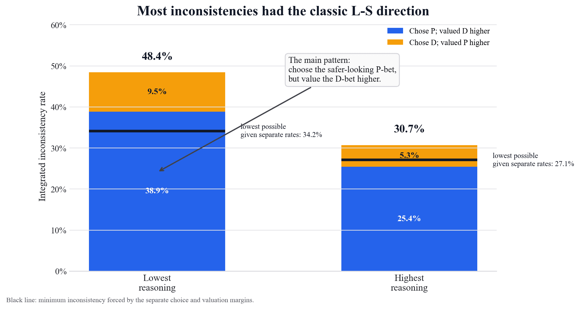
The total bar height is the inconsistency rate. The black line is the lower bound, the disagreement forced by the observed margins. The dominant component was the classic L-S direction. In the primary format, total inconsistency fell from 48.4% to 30.7% when comparing the lowest reasoning settings with the highest. The choose-P/price-D-higher component fell from 38.9% to 25.4%. The opposite direction was smaller: 9.5% at the lowest settings and 5.3% at the highest. The lower bound also fell, from 34.2% to 27.1%, which means the choice and valuation margins themselves became more aligned under the highest reasoning settings. The result is not just an artifact of independently pairing noisy samples.
Was the inconsistency observed in all models?
The following figure shows the primary-format result by model.
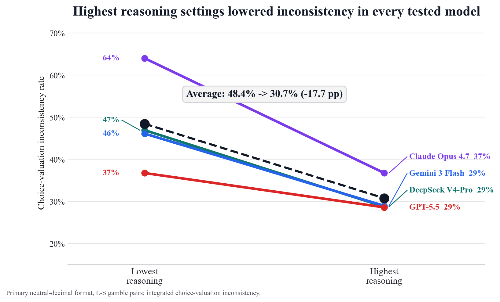
Every tested model moved in the same direction: lower inconsistency at the highest provider-exposed reasoning setting. But the inconsistency remained substantial, and the effect size varied. Anthropic showed the largest reduction, OpenAI the smallest, with DeepSeek and Google in between. Since provider reasoning settings are bundles, not clean mechanisms, and each model is governed by provider-side policies that vary, the result can only speak to the effect of changing provider-exposed reasoning settings under these specific conditions.
Could this be caused by refusals, parsing, or display order?
Probably not. The study was preregistered, API calls were interleaved among providers, all planned calls completed, display order was exactly balanced, and there were no full refusals. There were 9 parse failures total, and the experiment did not use content retries to repair malformed answers.
Is response length to blame?
Potentially. On primary L-S rows, the highest reasoning settings produced about 10 times more visible output tokens on average: 452.4 versus 47.3. That could matter. But output length is not a complete explanation: Gemini’s visible output length did not increase, moving from 52.1 tokens at the lowest setting to 47.9 at the highest, while the high setting still reported reasoning-token metadata.
What might be going on?
One possibility is that choice and pricing may emphasize different attributes. A direct-choice prompt can make high probability more salient; a selling-price prompt can make the larger payoff more salient. That is the classic scale-compatibility story.[4]
Another possibility is mode mixture or task recognition. The model may sample different coherent response modes under different prompts, and each individual response mode might be internally coherent even if the distribution is not. Or the model may have learned patterns from preference-reversal examples. This study cannot separate those mechanisms.
What are the practical implications?
Do not assume a model has one stable preference ordering just because each individual API call is reasonable. If a system uses LLMs to both recommend options and assign scores, prices, bids, rankings, or thresholds, audit those formats together during consistency testing. And do not rely on the highest reasoning settings as a sole mitigation.
What are some ideas for follow-up studies and next steps?
- A same-session paired study, with task order counterbalanced, to see if the distributional result occurs within sessions.
- A crossed response-budget study that separates reasoning setting from visible output length.
- A paradigm-recognition study using noncanonical gambles.
- Better null models for separating random instability from systematic preference-reversal-style structure.
If you’ve come this far, thank you for reading. I created this post because I honestly do not know what to make of the results (or the methodology) and would appreciate any and all feedback. The preregistration details and GitHub repo, which includes the preprint, can be found below (the paper is still very much a work in progress).
Materials:
- Preregistration: OSF unified study page, DOI 10.17605/OSF.IO/ACBS3
- GitHub repository: jondangresearch/llm-inconsistency
- ^
Sarah Lichtenstein and Paul Slovic, “Reversal of Preferences Between Bids and Choices in Gambling Decisions,” Journal of Experimental Psychology 89(1):46-55, 1971, https://doi.org/10.1037/h0031207; Sarah Lichtenstein and Paul Slovic, “Response-Induced Reversals of Preference in Gambling: An Extended Replication in Las Vegas,” Journal of Experimental Psychology 101(1):16-20, 1973, https://doi.org/10.1037/h0035472.
- ^
Amos Tversky, Paul Slovic, and Daniel Kahneman, “The Causes of Preference Reversal,” American Economic Review 80(1):204-217, 1990, https://www.jstor.org/stable/2006743.
- ^
For readability, I write exact ties here; the preprint uses a 25-cent tie band so as not to treat quarter-scale rounding differences as real preferences. This tolerance is small relative to the outcome scale, with the maximum outcomes ranging from $10.04 to $32.65.
- ^
Paul Slovic, Dale Griffin, and Amos Tversky, “Compatibility Effects in Judgment and Choice,” in Insights in Decision Making, 1990, https://hdl.handle.net/1794/22403. See also Amos Tversky, Shmuel Sattath, and Paul Slovic, “Contingent Weighting in Judgment and Choice,” Psychological Review 95(3):371-384, 1988, https://doi.org/10.1037/0033-295X.95.3.371.
Discuss