L2 distance told me two audio fingerprints were similar. They weren’t. The problem wasn’t my model. It was the metric.
If you have not read my last blog on vector index, it will help you understand why I am doing what I am doing.
Access this story for free here
The Problem With L2
OmniPulse revolves around WST fingerprints. They aren’t a single point in space. They are the distribution of energy across wavelet scales and time. Two fingerprints can have similar energy overall but very different structure. L2 on the flattened array measures “are these numbers similar?” It doesn’t measure “are these distributions similar?” That’s the wrong question.
What I needed was a distance that can measure how much work it takes to transform one distribution into another. That’s exactly what Wasserstein distance measures. And specifically, Sliced-Wasserstein is a version that’s fast enough to actually use.
What Wasserstein Distance Actually Is
Let’s understand the Wasserstein distance with an analogy. Imagine two piles of dirt on the ground. Wasserstein distance asks what’s the minimum amount of work to move one pile so it looks like the other? Work equals mass times distance moved. If the piles are in the same place, zero work. If they’re far apart, lots of work.
Now for distributions we just replace “piles of dirt” with “distributions of energy.” Two audio fingerprints have different energy patterns across wavelet scales. Wasserstein measures how much you’d have to rearrange the energy in fingerprint A to make it look like fingerprint B.
The problem with L2 is that it compares coordinate by coordinate and asks “is coefficient 47 of fingerprint A close to coefficient 47 of fingerprint B?” It doesn’t care that coefficient 47 of A might be semantically similar to coefficient 52 of B. But on the other hand Wasserstein finds the optimal matching, it pairs up the energy across both fingerprints in the most efficient way possible.
Wasserstein is beautiful mathematically but it’s also O(N³) to compute. For N=1000 points that’s a billion operations. Unusable at scale. That’s where slicing comes in.
The Slicing Trick
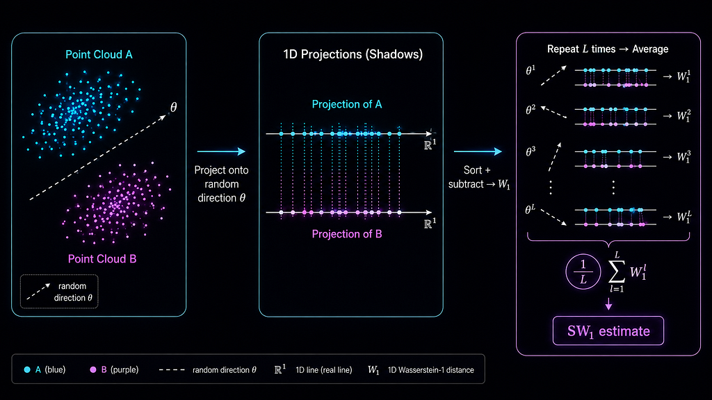
The problem with exact Wasserstein in high dimensions is that there isn’t any natural ordering so you can’t sort points in 2D or higher the only way you can do is in 1D. In 1D, Wasserstein has a beautiful closed-form solution: sort both distributions, subtract by rank, average.O(N log N). Fast.
Sliced-Wasserstein exploits this. Project both point clouds onto a random 1D direction (a unit vector). Now you have two 1D distributions. Compute exact Wasserstein in 1D, sort and subtract. Do this for L random directions and average. That average is the Sliced-Wasserstein estimate.
Why does this work? By the law of large numbers, as L grows the average converges to the true Wasserstein distance (in expectation). More projections = better estimate, less variance. The cost per projection is O(N log N) is just a sort. Total cost: O(L × N log N). For N=1000, L=100: about a million operations instead of a billion. Three orders of magnitude faster.
Each projection is a dot product that means signal · direction gives a single number, the shadow of the point onto that line. You’re collapsing a high-dimensional distribution onto a 1D line, measuring the 1D distance, and averaging over many such lines.
The Implementation
The API is three pieces. First, configure the estimator:
let sw = SlicedWasserstein::new(SwConfig {
    dim: 64,
    n_projections: 100,
    seed: 42,
});
dim is the dimensionality of each point in the cloud and not the total float count. For N points each living in ℝ⁶⁴, dim=64. n_projections is L which is the number of random directions. More projections means a better estimate at linear cost. seed pins the random directions so results are deterministic across runs: same seed, same directions, same distances.
The input type is PointCloud, not a raw Vec<f32>. A flat array is ambiguous like 1024 floats could be one point in ℝ¹⁰²⁴ or 16 points in ℝ⁶⁴. PointCloud::new(data, dim) makes the structure explicit and validates at construction that data.len() % dim == 0.
let cloud = PointCloud::new(data, 64)?;
Once you have point clouds, distance is one call:
let dist = sw.distance(cloud_a.data(), cloud_b.data());
Projections are cached at construction, not regenerated per call. That means distance(a, b) returns bit-identical results every time which matters for HNSW, where the index contract requires the metric to be consistent across calls. To plug SW₁ directly into the HNSW index from vector-index:
let mut index = HnswIndex::new(sw, HnswConfig::default());
index.insert(cloud)?;
Correctness Guarantees
The implementation verifies six properties that any correct Wasserstein estimator must satisfy. The strongest signal is the 1D ground truth test: in 1D Sliced-Wasserstein equals the exact Wasserstein because there’s only one direction to project onto. So you can verify against a known analytic answer, if distance([0, 1], [0.5]) returns 0.5, the implementation is numerically correct, not just structurally plausible. That’s the difference between “it compiled and ran” and “the math is right.”
The other five properties follow from the geometry. Self-distance is bit-exact zero and not approximately zero because projecting a distribution onto itself produces identical sorted arrays and every term cancels. Symmetry holds because the absolute value in the 1D Wasserstein formula means swapping inputs doesn’t change the area between CDFs. Translation invariance means distance(a + t, b + t) == distance(a, b) for any shift, moving both distributions by the same amount doesn’t change how different they are. Scale equivariance means distance(λa, λb) == λ × distance(a, b) scaling both scales the distance proportionally. And the random projection directions are generated using Marsaglia’s method: sample from a multivariate Gaussian, then normalize. The Gaussian is spherically symmetric, so the normalized result is uniform on the sphere. Sampling uniformly in a cube and normalizing is the common mistake and it oversamples the corners and biases the estimate.
Real Results

To test whether the metric was actually capturing signal structure, I stored five fingerprints in OmniPulse’s HNSW index: silence (344 zeros), a low-frequency sine wave (ω=0.01), a high-frequency sine wave (ω=1.0), a mid-band sine wave (ω=0.1), and Gaussian noise. Then I queried against silence and looked at what came back.
zeros → zeros: 0.000000
zeros → sine-low: 0.001942
zeros → sine-high: 0.002710
zeros → sine-mid: 0.008654
zeros → noise-42: 0.026856
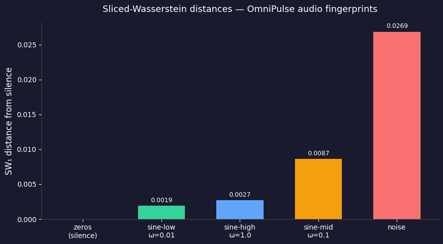
The ordering tells a physically coherent story. Gaussian noise is the most distant from silence and it activates every scattering path simultaneously, spreading energy across the entire wavelet plane. The low-frequency sine is the closest at ω=0.01 it barely completes half a cycle across the signal window, so it scatters almost like a flat signal. The mid-band sine lands in between, spreading energy across more paths than either extreme. The metric didn’t just return numbers, it also returned numbers that make physical sense.
This is what a geometrically correct metric looks like in practice. L2 on the flattened fingerprints would have returned different distances, and they wouldn’t have this ordering. The Wavelet Scattering Transform produces distributions on the wavelet plane. Sliced-Wasserstein measures distance between distributions. The two compose correctly and the distance table above is the proof.
When to Use It
Use SW₁ when your data is naturally a distribution or a set of points, not a single vector. Point clouds (LiDAR scans, 3D models, molecular conformations), document distance where a document is a bag of word embeddings, video retrieval where a video is a distribution over frame embeddings, single-cell genomics where each cell is a distribution over gene expression, generative model evaluation where you’re comparing real vs generated sample distributions. If you’re comparing two Vec<f32> embeddings from a language model, use cosine because SW₁ is solving a different problem.
What’s Missing in v0.1.0
Only W₁ is implemented, W₂ (quadratic cost) is not. Weighted distributions with explicit masses (histograms) aren’t supported yet; the current implementation assumes uniform mass per point. These are on the roadmap but not in 0.1.0.
sliced-wasserstein is on crates.io:
cargo add sliced-wasserstein
The vector-index post covers the retrieval side as in “how HNSW finds nearest neighbors in O(log N)”. This post covers the metric side as in what “nearest” actually means for distributions. Together they’re the retrieval layer of OmniPulse, running in production on real audio signals.
L2 Distance was Giving Me Wrong Answers. Here’s the Metric That Fixed it. was originally published in Towards AI on Medium, where people are continuing the conversation by highlighting and responding to this story.