How ChatGPT Works Explained With Minimal Python Knowledge

A Deep Dive into Andrej Karpathy’s microGPT Implementation

In the world of artificial intelligence, Andrej Karpathy is a well-known figure. He has worked at Stanford, led AI efforts at Tesla, and contributed to OpenAI. Beyond that, he has a rare talent for explaining complex ideas clearly and engagingly.

One of his recent projects, microGPT, is a perfect example of that clarity.

At first glance, it might seem impossible: a working GPT model implemented in roughly 200 lines of Python. Yet this is exactly what microGPT is. The code is not compressed or cryptic; it is readable, structured, and carefully commented. Even more interesting, it avoids relying on large external frameworks, meaning it includes both the model and the minimal infrastructure needed to train it.

It’s not even a full repository, just a single GitHub Gist.

This article explores how this compact implementation works and, more importantly, what it reveals about modern language models.

What “GPT” Really Means

GPT stands for Generative Pretrained Transformer. This architecture lies at the core of most modern large language models. Even ChatGPT carries this term in its name, and many of today’s leading alternatives rely on the same fundamental concept.

At its heart, a GPT model works by predicting the next word (or token) based on the words that came before it.

In fact, this is the basic mechanism behind all language models. They generate text step by step: first predicting the next word, then appending it to the sequence, then predicting the next one again, and repeating this process continuously.

At first, this might sound almost trivial. But if we look closer, accurately predicting the next word requires a surprising degree of understanding of context, structure, and meaning.

Inside a neural network, this apparent “reasoning” is actually implemented as a massive mathematical function.

The input text is first converted into numerical form, then passed through this function, which outputs the most likely next word. In theory, any rule-based system can be expressed mathematically like this. The challenge is to find a function that successfully captures the patterns of human language.

This function is what we refer to as the model.

The difficulty is that such functions can become extraordinarily complex. Modern language models often contain billions of parameters, meaning the underlying mathematical representation consists of billions of adjustable elements. Designing or managing something like this by hand would be completely impractical.

Fortunately, there’s a smarter approach.

Instead of explicitly defining the full function, we start with a flexible structure — a kind of template — with many tunable parameters. These parameters are then automatically adjusted until the model produces useful results.

Different types of problems use different kinds of templates:

• Convolutional networks are typically applied to image-related tasks
• MLPs (multi-layer perceptrons) are used for general-purpose function approximation
• Transformers power language models like ChatGPT
• and many others

Each of these architectures represents a large mathematical framework capable of approximating complex patterns — once its parameters are properly tuned.

Which brings us to the key question: how do we actually tune them? In other words, how do we “program” a neural network?

How Neural Networks Learn: Gradient Descent Explained

Manually tuning the parameters of a neural network is clearly not an option — especially when we’re dealing with models that have millions or even billions of adjustable values.

Instead, this process is automated using data. We call it training, and the key technique behind it is gradient descent.

Given a large dataset and a complex mathematical model, we can measure how well the model performs by calculating its error on each example.

For transformer-based models, the process looks roughly like this:

Words are mapped into a high-dimensional vector space, where similar words are positioned closer together. In this representation, every word corresponds to a point in that space.

The model takes a sequence of words as input and predicts the next one. Since both predicted and actual words are represented as vectors, we can measure the difference between them. This difference gives us a numerical value for the error.

And this is where things get interesting.

With gradient descent, we can determine how to adjust the model’s parameters in order to reduce that error.

If we have enough training data, a sufficiently large model, and enough training time, the system gradually aligns itself with the patterns in the data, producing increasingly accurate predictions.

But what’s really happening under the hood? How does gradient descent actually discover better parameter values?

We can think of the error as defining a function over a high-dimensional space, where each dimension corresponds to one parameter of the model.

Since imagining such a space is beyond human intuition, it helps to simplify it into a familiar analogy: a landscape filled with hills and valleys.

In this picture:

• Each point represents a specific configuration of parameters
• The elevation at that point represents the model’s error
• Lower regions correspond to better-performing models

At the start of training, the parameters are initialized randomly — like being dropped somewhere on this landscape without any prior knowledge.

The objective is to reach the lowest possible point, where the error is minimized.

The challenge is that we cannot see the landscape. It’s like trying to descend a mountain while blindfolded, or navigating through dense fog.

So how do we proceed?

This is exactly where gradient descent comes into play.

In mathematics, the derivative tells us the slope of a function at a given point — in other words, which direction leads downhill.

Gradient descent uses this idea in a simple loop:

• Estimate the slope at the current position
• Take a small step in the direction that reduces the error
• Repeat the process

By iterating this over and over, the model gradually moves toward lower and lower regions of the error landscape.

That’s essentially the whole idea behind gradient descent.

But one important question remains: how do we compute the slope for such a massive and complex function?

Without going too deep into the math (there are excellent explanations out there, including detailed walkthroughs by Andrej Karpathy), the key insight is this:

Every mathematical operation has a known way to compute its local gradient. Using the chain rule, we can combine these local gradients to calculate the gradient of the entire function.

The trick is to traverse the sequence of operations in reverse, accumulating gradients along the way. This method is known as backpropagation.

All major deep learning frameworks handle this automatically.

For example:

• TensorFlow uses a system called GradientTape, which records operations so gradients can be computed afterward
• PyTorch uses autograd, where each tensor tracks how it was created, enabling automatic gradient computation

These tools make it possible to train massive neural networks without ever manually touching the underlying mathematics.

A Tiny Autograd Engine: How Karpathy’s Implementation Works

Andrej Karpathy’s implementation follows exactly the principles we discussed — just in an extremely compact and elegant form. Let’s take a closer look at how it works.

# Let there be Autograd to recursively apply the chain rule through a computation graph
class Value:
    __slots__ = ('data', 'grad', '_children', '_local_grads') # Python optimization for memory usage

    def __init__(self, data, children=(), local_grads=()):
        self.data = data                # scalar value of this node calculated during forward pass
        self.grad = 0                   # derivative of the loss w.r.t. this node, calculated in backward pass
        self._children = children       # children of this node in the computation graph
        self._local_grads = local_grads # local derivative of this node w.r.t. its children

    def __add__(self, other):
        other = other if isinstance(other, Value) else Value(other)
        return Value(self.data + other.data, (self, other), (1, 1))

    def __mul__(self, other):
        other = other if isinstance(other, Value) else Value(other)
        return Value(self.data * other.data, (self, other), (other.data, self.data))

    def __pow__(self, other): return Value(self.data**other, (self,), (other * self.data**(other-1),))
    def log(self): return Value(math.log(self.data), (self,), (1/self.data,))
    def exp(self): return Value(math.exp(self.data), (self,), (math.exp(self.data),))
    def relu(self): return Value(max(0, self.data), (self,), (float(self.data > 0),))
    def __neg__(self): return self * -1
    def __radd__(self, other): return self + other
    def __sub__(self, other): return self + (-other)
    def __rsub__(self, other): return other + (-self)
    def __rmul__(self, other): return self * other
    def __truediv__(self, other): return self * other**-1
    def __rtruediv__(self, other): return other * self**-1

    def backward(self):
        topo = []
        visited = set()
        def build_topo(v):
            if v not in visited:
                visited.add(v)
                for child in v._children:
                    build_topo(child)
                topo.append(v)
        build_topo(self)
        self.grad = 1
        for v in reversed(topo):
            for child, local_grad in zip(v._children, v._local_grads):
                child.grad += local_grad * v.grad

In this implementation, the entire gradient computation mechanism is packed into a single class called Value, spanning only a few dozen lines.

This class wraps a numerical value, but also carries additional information:

• which earlier values it depends on (its children)
• and the local gradients required for backpropagation

If you scan through the code, you’ll notice that standard mathematical operators are overridden:

• __add__
• __mul__
• and several others

This means that every time we operate on Value objects, the system not only computes the result, but also builds a computation graph and stores how gradients should flow through it.

The backward() method is where everything comes together. It traverses this graph in reverse order and accumulates gradients step by step, ultimately computing how each value contributed to the final error.

And that’s really the essence of automatic differentiation.

But computing gradients is only half of the story. We also need a way to use them to improve the model.

This is where optimization comes in — specifically, gradient descent.

# Adam optimizer update: update the model parameters based on the corresponding gradients
    lr_t = learning_rate * (1 - step / num_steps) # linear learning rate decay
    for i, p in enumerate(params):
        m[i] = beta1 * m[i] + (1 - beta1) * p.grad
        v[i] = beta2 * v[i] + (1 - beta2) * p.grad ** 2
        m_hat = m[i] / (1 - beta1 ** (step + 1))
        v_hat = v[i] / (1 - beta2 ** (step + 1))
        p.data -= lr_t * m_hat / (v_hat ** 0.5 + eps_adam)
        p.grad = 0

In this case, Karpathy uses the Adam optimizer — one of the most popular optimization methods in deep learning.

Unlike basic gradient descent, Adam adjusts the step size dynamically by keeping track of past gradients. This typically leads to faster convergence and more stable training.

Together, these two pieces — gradient computation and parameter updates — form what we might call the “engine” of deep learning.

No matter the application — whether it’s a language model, an image generator, a robotics system, or an autonomous vehicle — the training process follows this same fundamental pattern.

What’s remarkable is that this entire idea can be expressed in just a few lines of Python.

Of course, production-grade frameworks like TensorFlow, PyTorch, or JAX provide highly optimized implementations that run on GPUs, TPUs, and distributed systems, along with many additional improvements.

But at their core, they all rely on exactly the same principle demonstrated by this minimal example.

A Tiny GPT Model: How Karpathy’s Implementation Works

As mentioned earlier, the core objective of GPT is to predict the next token based on the preceding ones.

This description is slightly simplified because the input isn’t made up of words in the traditional sense, but of tokens.

Tokens are similar to words, but they are more flexible. Instead of relying on a fixed dictionary, the model builds its vocabulary statistically from the training data. In practice, tokens are recurring character sequences that frequently appear in the dataset.

This means training doesn’t start with a predefined mapping of words to numbers. Instead, the vocabulary itself is discovered during preprocessing.

This approach is particularly powerful for agglutinative languages like Hungarian, where a single word can take many different forms due to suffixes and grammatical variations.

With enough data, a language model can learn to represent virtually any language — natural or artificial.

In fact, tokens don’t even have to represent text. They can encode:

• parts of images
• segments of audio
• sensor measurements
• or almost any structured data

Because of this, transformer models are not limited to text. The same underlying architecture can be applied to image generation, speech recognition, robotics, and beyond.

In Karpathy’s example, however, the model is intentionally kept very small. Instead of working with words or subword tokens, it operates at the character level.

Its goal is therefore much simpler: not to generate full sentences, but to produce realistic-looking names.

The training data consists of a large collection of names, and after training, the model should be able to generate new ones that statistically resemble the originals.

Of course, this is far from something like ChatGPT. But the difference is mostly about scale rather than principle.

If we expanded this tiny model by several orders of magnitude, switched from characters to tokens, and trained it on massive internet-scale datasets, we would arrive at something very similar to modern large language models.

In practice, such models are typically trained in two phases:

• Pretraining — learning general language patterns from vast amounts of raw text
• Fine-tuning — refining the model using curated, human-generated data to improve usefulness and alignment

This process requires enormous computational resources and high-quality datasets, often costing millions in infrastructure.

Since most of us don’t have access to that kind of setup, we’ll stick to generating names.

# Let there be a Dataset `docs`: list[str] of documents (e.g. a list of names)
if not os.path.exists('input.txt'):
    import urllib.request
    names_url = 'https://raw.githubusercontent.com/karpathy/makemore/988aa59/names.txt'
    urllib.request.urlretrieve(names_url, 'input.txt')
docs = [line.strip() for line in open('input.txt') if line.strip()]
random.shuffle(docs)
print(f"num docs: {len(docs)}")

# Let there be a Tokenizer to translate strings to sequences of integers ("tokens") and back
uchars = sorted(set(''.join(docs))) # unique characters in the dataset become token ids 0..n-1
BOS = len(uchars) # token id for a special Beginning of Sequence (BOS) token
vocab_size = len(uchars) + 1 # total number of unique tokens, +1 is for BOS
print(f"vocab size: {vocab_size}")

At the start of the code, we load the dataset of names and construct the vocabulary.

In this minimal setup, the vocabulary is simply the set of unique characters found in the dataset.

Each character is then assigned a numerical ID, allowing the text to be converted into a sequence of numbers that the neural network can process.

Embeddings: Turning Tokens into Meaningful Vectors

The concept of embeddings itself is quite straightforward, yet incredibly powerful.

Instead of feeding raw token IDs into the model, we transform each token into a point in a high-dimensional vector space. These vectors are what the neural network actually operates on.

In fact, you can think of any neural network as a function that maps vectors from one high-dimensional space into another.

For example:

• In an image classifier that distinguishes between dogs and cats, the network maps an image into a space where one axis represents “dogness” and another represents “catness”
• In an image generation system like Midjourney, the model transforms random noise into a structured high-dimensional representation corresponding to an image guided by a prompt

No matter the application, the underlying idea is the same: a large mathematical function transforms vectors into other vectors.

GPT follows this exact pattern.

The dimensionality of this vector space is defined by the parameter n_embd, which in this implementation is set to 16.

This means that each token — here, each character — is represented as a 16-dimensional vector.

Mathematically, this transformation is just a matrix multiplication.

In the code, the matrix responsible for mapping tokens into vectors is called wte (token embeddings).

However, knowing which characters appear is not sufficient. Their order also carries meaning.

If we rearrange the characters in a sequence, the meaning can change entirely.

To account for this, the model introduces positional information through another embedding matrix called wpe.

Both the token identity and its position are mapped into vectors of the same dimension, and these vectors are then added together.

The result is a single vector that captures both:

• what the token is
• where it appears in the sequence

Earlier, we mentioned that these vector representations need to be meaningful because the model later measures error based on distances between vectors.

Ideally:

• Almost correct predictions should be close to the target vector
• Completely wrong predictions should be far away

This leads to an interesting question: how do we design such a space?

Surprisingly, we don’t design it at all.

Instead, both embedding matrices (wte and wpe) are initialized with random values, and gradient descent gradually shapes them during training.

Given enough data, the model learns to organize this space in a way that captures useful relationships.

And this is where things get fascinating.

In models like word2vec, simple vector arithmetic can reflect semantic relationships. A well-known example is:

king − man + woman ≈ queen

This shows that the embedding space begins to encode a simplified structure of the world, where relationships between concepts emerge as geometric patterns between vectors.

Transformer: The Engine Behind GPT

Now that we understand how tokens are turned into vectors, we can finally look at the neural network itself — the component that transforms these vectors into new ones representing the next token.

In essence, the model takes vectors from the embedding space and maps them back into the same space, but shifted forward by one position. For each token, it predicts which token is most likely to come next. By repeating this process step by step, the model can generate an entire sequence — whether that’s a sentence, a paragraph, or, in our case, a name.

The architecture that makes this possible is called the Transformer.

It was introduced in 2017 by researchers at Google in the landmark paper Attention Is All You Need.

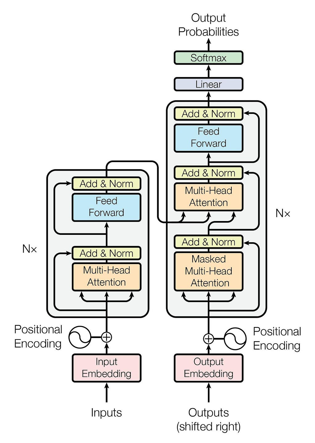
The original Transformer architecture was designed for machine translation and consisted of two main parts:

• an encoder, which processes the input sequence
• a decoder, which generates the output sequence

However, for generative models like GPT, only half of this setup is required: the decoder.

This is why GPT models are often described as decoder-only transformers.

The decoder takes the input tokens and passes them through a stack of identical layers. Each layer contains two key components:

• Self-attention
• a feed-forward neural network (MLP)

In larger models, these layers are repeated many times. In architectural diagrams, this is usually shown as ×N, meaning the same block is stacked repeatedly to increase the model’s capacity.

One of the most important innovations of the Transformer is how it processes sequences.

Earlier models, such as recurrent neural networks (RNNs), handled text step by step, passing information along sequentially from one token to the next.

Transformers take a completely different approach.

They process the entire sequence at once, allowing the model to directly learn relationships between the tokens.

This capability comes from the attention mechanism, which lets the model decide which parts of the input are most relevant when making predictions.

And that’s exactly why the original paper was titled Attention Is All You Need.

Attention: How Transformers Understand Context

The attention mechanism determines how relevant each token is to every other token in a sequence.

For each token vector, the model computes a set of weights that indicate how much attention it should give to the other tokens. It then aggregates information from those tokens accordingly.

As a result, the updated vector no longer represents just the token itself — it encodes its meaning within the full context of the sequence.

This might sound abstract, but the intuition is quite simple.

Imagine asking a model: “What is the capital of France?”

Looking at the word “capital” alone isn’t enough to answer the question. But attention allows the model to connect it with “France”, forming a contextual understanding of the phrase “capital of France”. This enables the model to produce the correct answer: Paris.

One useful way to think about transformers is as a kind of “soft database.”

Instead of storing explicit facts, the model encodes knowledge in a high-dimensional vector space. Because neural networks approximate patterns rather than memorize exact rules, they can often generalize to questions they’ve never seen before.

Going back to our earlier embedding example: if the model has learned about kings and women, it may still infer something about queens, because these relationships are captured geometrically in the embedding space.

If we stretch this database analogy a bit:

• Attention acts like a search mechanism, helping the model find relevant pieces of information
• The MLP layers contain and transform the knowledge itself

This is, of course, only an intuition — not a literal description.

In real transformer models like ChatGPT, these attention and MLP blocks are stacked many times. Knowledge is distributed across layers rather than stored in a single place.

Each layer also includes residual connections, which mix the original input with the transformed output. This helps stabilize training and allows information to flow more effectively through the network.

As vectors move through these layers, increasingly abstract representations emerge. By the final layer, the model has combined information from multiple levels of processing.

The full process is far too complex to follow step by step — but remarkably, it works.

Now that we have a high-level intuition, let’s look at how attention is implemented in code.

 # 1) Multi-head Attention block
        x_residual = x
        x = rmsnorm(x)
        q = linear(x, state_dict[f'layer{li}.attn_wq'])
        k = linear(x, state_dict[f'layer{li}.attn_wk'])
        v = linear(x, state_dict[f'layer{li}.attn_wv'])
        keys[li].append(k)
        values[li].append(v)
        x_attn = []
        for h in range(n_head):
            hs = h * head_dim
            q_h = q[hs:hs+head_dim]
            k_h = [ki[hs:hs+head_dim] for ki in keys[li]]
            v_h = [vi[hs:hs+head_dim] for vi in values[li]]
            attn_logits = [sum(q_h[j] * k_h[t][j] for j in range(head_dim)) / head_dim**0.5 for t in range(len(k_h))]
            attn_weights = softmax(attn_logits)
            head_out = [sum(attn_weights[t] * v_h[t][j] for t in range(len(v_h))) for j in range(head_dim)]
            x_attn.extend(head_out)
        x = linear(x_attn, state_dict[f'layer{li}.attn_wo'])
        x = [a + b for a, b in zip(x, x_residual)]

In Karpathy’s implementation, attention is built using three matrices:

• Q (Query)
• K (Key)
• V (Value)

These matrices project each token vector into three different representations.

For every token, the model computes:

• a query vector
• a key vector
• a value vector

The query vector of a token is then compared to the key vectors of all tokens in the sequence.

This comparison is done using a dot product, which produces a score indicating how strongly two tokens are related.

These scores are then passed through the softmax function, turning them into probabilities that sum to 1. These probabilities determine how much attention each token receives.

Finally, the model combines the value vectors using these attention weights, producing a new vector that integrates information from across the sequence.

The core formula for this process is:

Attention(Q, K, V) = softmax(QKᵀ / √dₖ) V

Where:

• QKᵀ computes the similarity between queries and keys
• √dₖ is a scaling factor that stabilizes training
• softmax converts the scores into attention probabilities
• V provides the information that is combined according to those probabilities

The result is a context-aware representation for each token.

At this point, it’s important to introduce another key concept: context length.

Because transformers compare every token with every other token, the computational cost grows quadratically with sequence length.

If you double the number of tokens, the computation roughly quadruples.

This makes context length one of the main limitations of transformer models.

Unlike some other architectures, transformers don’t have a persistent memory. They can only operate on the tokens within their current context window. Anything outside that window is effectively invisible.

To work around this limitation, many modern systems use external memory.

A common approach is to store information in a vector database. When a query comes in, the system:

• converts the query into a vector
• retrieves relevant information from the database
• injects that information into the model’s context

This allows the model to generate answers based on both the question and the retrieved knowledge.

This technique is known as Retrieval-Augmented Generation (RAG) and is widely used in modern AI systems.

In such setups, the model doesn’t need to store all knowledge internally — it only needs to reason over the information available in its context.

But this still depends on available context space, which is why context length remains a critical factor.

Returning to Karpathy’s implementation, the model uses multi-head attention, an extension of the basic attention mechanism.

Instead of using a single set of Q, K, and V matrices, the model uses multiple attention heads — in this case, four.

Each head learns to focus on different types of relationships. One might capture short-range dependencies, while another focuses on broader contextual patterns.

To keep computation manageable, each head operates in a lower-dimensional space.

Earlier, we worked in a 16-dimensional space. With four heads, each head operates on 4-dimensional vectors. The outputs of all heads are then combined back into a single vector.

Even though each head is smaller, their combined output is typically more expressive and more powerful than a single attention mechanism.

The MLP Block: Where the Transformation Happens

Now that we’ve explored attention, we can move on to the second key component of a transformer block: the MLP, or feed-forward neural network.

In the code, the MLP section looks like this:

 # 2) MLP block
        x_residual = x
        x = rmsnorm(x)
        x = linear(x, state_dict[f'layer{li}.mlp_fc1'])
        x = [xi.relu() for xi in x]
        x = linear(x, state_dict[f'layer{li}.mlp_fc2'])
        x = [a + b for a, b in zip(x, x_residual)]

An MLP is one of the most classic neural network architectures. If we examine the weight matrices, we can think of each row as representing a neuron.

A neuron is a simple computational unit that:

• multiplies each input by a weight
• sums those weighted inputs
• applies a nonlinear activation function to produce an output

This concept was originally inspired by biological neurons in the human brain. Early neural network research aimed to mimic how the brain might process information.

However, modern AI systems have evolved far beyond this biological analogy.

In components like the MLP, we can still loosely recognize neuron-like behavior. But in mechanisms such as attention, the connection to biological brains becomes much less clear.

Because of this, it’s often more accurate to think of modern neural networks as highly flexible mathematical functions rather than literal brain simulations.

Looking at the code, the MLP block follows a simple three-step structure:

1. A linear transformation (matrix multiplication)
2. A nonlinear activation function (ReLU)
3. Another linear transformation

Despite its simplicity, this structure has a very powerful property.

MLPs are known as universal approximators. This means that, given enough capacity, they can approximate almost any mathematical function to arbitrary precision.

In theory, a single massive MLP could learn extremely complex patterns.

In practice, however, that wouldn’t be very efficient.

That’s why transformer architectures combine multiple components — like attention, MLP layers, and deep stacking — to distribute computation and learning more effectively across the network.

From Probabilities to Text: Sampling and Temperature

The output of the network is not a single token, but a probability distribution over all possible tokens.

In other words, for every token in the vocabulary, the model assigns a probability indicating how likely it is to appear next in the sequence.

When generating text, the model doesn’t simply pick the top option every time. Instead, it samples from this distribution.

This means that tokens with higher probabilities are more likely to be selected, but there is still some randomness involved.

This randomness is controlled by a parameter known as temperature.

Temperature determines how deterministic — or how creative — the model’s output will be.

• Low temperature → the model heavily favors the most likely tokens, leading to more predictable and precise outputs
• High temperature → the probability distribution becomes more spread out, allowing less likely tokens to be chosen, which increases diversity and creativity

For example:

• If the goal is to analyze a document or answer factual questions, a lower temperature is usually preferred
• If the goal is to generate creative writing or explore ideas, a higher temperature can produce more varied and interesting results

In this way, temperature acts as a simple but powerful control knob, letting us adjust the balance between accuracy and creativity in the model’s behavior.

Wrapping Up: From Code to Understanding

This is roughly what I set out to explain about this elegant piece of code — and about GPT models more broadly.

In several places, the explanation had to remain somewhat high-level. The goal was to find a balance between depth and readability: to share meaningful insights while keeping everything within the scope of a single article.

If some parts felt a bit dense, or if you’d like to dive deeper into the details, I highly recommend exploring the work of Andrej Karpathy. His website, blog, and YouTube content offer clear and in-depth explanations of all the concepts covered here.

Hopefully, this article provided a useful overview — and perhaps sparked some curiosity along the way.

If nothing else, consider it an invitation to explore the fascinating world of AI just a little further.

---

How ChatGPT Works Explained With Minimal Python Knowledge was originally published in Towards AI on Medium, where people are continuing the conversation by highlighting and responding to this story.