GRU: The Simpler Successor to LSTM That Quietly Took Over Sequence Modeling

How GRU Simplified Memory Control While Preserving Long-Term Learning

LSTM solved one of the biggest failures in early recurrent neural networks: memory collapse over long sequences.

But after LSTM became successful, researchers noticed something uncomfortable.

The architecture worked well.
The architecture was also unnecessarily heavy.

Three gates.
Two separate memory systems.
Multiple matrix multiplications.
A large parameter count.

It solved the problem, but at a computational cost.

That led researchers to ask a new question:

Can we keep the memory advantages of LSTM while making the architecture simpler?

That question led to the creation of the Gated Recurrent Unit (GRU).

Introduced by Cho et al. in 2014, GRU became one of the most practical recurrent architectures ever designed.

Not because it was dramatically smarter than LSTM.

But because it achieved almost the same performance with a much simpler design.

And sometimes simplicity wins.

1. The Core Philosophy Behind GRU

LSTM treats memory as two separate systems:

• long-term memory → cell state (Cₜ)
• short-term memory → hidden state (hₜ)

GRU removes this separation.

Instead of maintaining two memory paths, GRU merges them into a single hidden state:

• hₜ

This hidden state now acts as both:

• working memory
• long-term memory

That simplification is the heart of GRU.

2. The Big Architectural Difference

LSTM

LSTM contains:

• Forget Gate
• Input Gate
• Output Gate
• Cell State
• Hidden State

GRU

GRU compresses this into:

• Update Gate
• Reset Gate
• Hidden State

No separate cell state.
No output gate.
Fewer parameters.
Faster training.

But the real question is:

How does GRU still preserve memory effectively with fewer components?

That is where the gates become important.

3. The Main Intuition Behind GRU

GRU is built around one central idea:

At every timestep, decide how much of the past should survive and how much new information should replace it.

That is all.

Everything inside GRU revolves around that decision.

The architecture achieves this using:

1. Update Gate (zₜ)
2. Reset Gate (rₜ)
3. Candidate Hidden State (h̃ₜ)

These three components together define the entire memory behavior of the network.

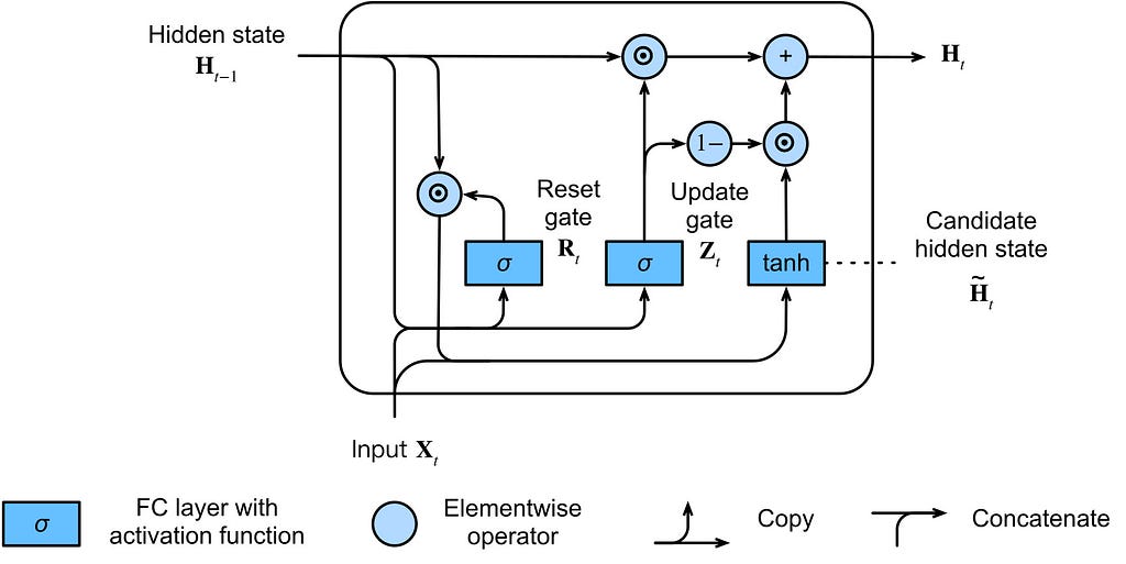
4. GRU Architecture Overview

At timestep (t), the GRU receives:

• previous hidden state: hₜ₋₁
• current input: xₜ

and produces:

• current hidden state: hₜ

Unlike LSTM, there is no separate cell state.

Everything happens directly through the hidden state.

5. Step 1: Reset Gate

The first gate inside GRU is the Reset Gate.

Formula:

• rₜ = σ(Wᵣ[hₜ₋₁, xₜ] + bᵣ)

Where:

• σ = sigmoid activation
• values lie between 0 and 1

6. Deep Intuition Behind the Reset Gate

The reset gate answers this question:

“How much of the previous memory should matter while creating new memory?”

This is extremely important.

Because sometimes old memory is useful.
Sometimes it becomes irrelevant.

The reset gate decides whether the model should:

• heavily depend on previous hidden state
• partially ignore previous context
• completely reset memory influence

That is why it is called the reset gate.

7. Intuition Example

Imagine this sentence:

“I grew up in France… Today I am learning Japanese.”

While processing “Japanese”, older information about “France” may not help much.

So the reset gate can suppress irrelevant past memory.

This allows the GRU to avoid dragging unnecessary historical context into the current computation.

8. What Happens Mathematically?

The reset gate directly affects candidate memory (later discussed) creation.

Specifically:

• h̃ₜ = tanh(Wₕ[rₜ ⊙ hₜ₋₁, xₜ] + bₕ)

Notice this term:

• rₜ ⊙ hₜ₋₁

This is the critical operation. (⊙ denotes element-wise multiplication)

The previous hidden state is filtered before being used.

That means:

• if rₜ ≈ 1
  → previous memory is preserved
• if rₜ ≈ 0
  → previous memory is mostly ignored

So the reset gate controls:

“How much past information should participate in forming the new candidate memory?”

9. Step 2: Candidate Hidden State

Now the GRU creates a possible new memory representation.

This is called the candidate hidden state.

Formula:

• h̃ₜ = tanh(Wₕ[rₜ ⊙ hₜ₋₁, xₜ] + bₕ)

This is one of the most important equations in GRU.

Because this is where the network creates:

• new understanding
• new context
• updated memory proposal

Think of (h̃ₜ) as:

“What the network thinks the memory should become.”

But this is still only a proposal.

The network has not committed to it yet.

That decision comes next.

10. Deep Intuition Behind the Candidate State

The candidate hidden state is not final memory.

It is a possible memory update.

You can think of it like this:

• hₜ₋₁ = old belief
• h̃ₜ = new proposed belief

The network now needs to decide:

Should I trust the old memory or replace it with the new one?

That decision is controlled by the update gate.

11. Step 3: Update Gate

Formula:

• zₜ = σ(W_z[hₜ₋₁, xₜ] + b_z)

The update gate is the most important gate in GRU.

This gate controls the balance between:

• old memory
• new memory

12. Deep Intuition Behind the Update Gate

The update gate answers this question:

“How much of the previous hidden state should survive into the future?”

This is the memory-preservation mechanism of GRU.

If:

• zₜ ≈ 1

then the model mostly keeps old memory.

If:

• zₜ ≈ 0

then the model mostly replaces memory using the candidate state.

So:

• high zₜ → preserve memory
• low zₜ → update aggressively

That is why the update gate behaves somewhat like a combination of:

• forget gate
• input gate

from LSTM.

GRU merged both ideas into a single gate.

That simplification is one of the reasons GRU is computationally lighter.

13. Step 4: Final Hidden State Update

Now comes the final memory update equation.

• hₜ = (1 − zₜ) ⊙ hₜ₋₁ + zₜ ⊙ h̃ₜ

This equation defines the entire behavior of GRU.

14. Understanding the Final Equation Deeply

You can also think of this equation as a soft interpolation between old and new memory, similar to how exponential moving averages smoothly combine past information with new observations.

This equation is essentially a weighted blend between:

• old memory
• new candidate memory

Break it down carefully.

First Term

(1 − zₜ)

This preserves previous memory.

If update gate is small:

• zₜ ≈ 0

then:

• (1 − zₜ) ≈ 1

So old memory dominates.

Second Term

zₜ ⊙ h̃ₜ

This injects new memory.

If:

• zₜ ≈ 1

then candidate memory dominates.

15. The Most Important Intuition in GRU

GRU never abruptly deletes memory.

Instead, it continuously interpolates between:

• old memory
• new memory

That smooth transition is one of the reasons GRUs train so effectively.

Instead of hard replacement:

GRU performs controlled memory blending.

That idea is extremely elegant.

16. Dimensional Understanding

Suppose:

• input dimension = 4
• hidden dimension = 3

Then:

• xₜ → (1 × 4)
• hₜ₋₁ → (1 × 3)

Concatenation:

• [hₜ₋₁, xₜ] → (1 × 7)

Weight matrices:

• Wᵣ, W_z, Wₕ → (7 × 3)

Outputs:

• rₜ, zₜ, h̃ₜ, hₜ → (1 × 3)

This dimensional consistency is important because recurrent architectures are ultimately controlled matrix transformations.

The “memory” emerges from the update dynamics.

17. Why GRU Works So Well

GRU works surprisingly well because it preserves the most important idea introduced by LSTM:

controlled gradient flow.

The update equation:

• hₜ = (1 − zₜ) ⊙ hₜ₋₁ + zₜ ⊙ h̃ₜ

contains an additive path.

That additive structure allows gradients to propagate more safely through time.

18. Gradient Intuition in GRU

Consider derivative flow through the hidden state.

From:

• hₜ = (1 − zₜ) ⊙ hₜ₋₁ + zₜ ⊙ h̃ₜ

The direct memory path contains:

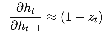
So:

• if (1 − zₜ) ≈ 1
  → old memory survives
• if (1 − zₜ) ≈ 0
  → network aggressively updates memory

This creates a controllable gradient path.

That is the reason GRU can maintain long-term dependencies without needing an explicit separate cell state.

19. Comparing GRU and LSTM

| Feature                 | LSTM   | GRU    |
|-------------------------|--------|--------|
| Separate cell state     | Yes    | No     |
| Hidden state            | Yes    | Yes    |
| Forget gate             | Yes    | No     |
| Input gate              | Yes    | No     |
| Output gate             | Yes    | No     |
| Update gate             | No     | Yes    |
| Reset gate              | No     | Yes    |
| Parameter count         | Higher | Lower  |
| Training speed          | Slower | Faster |
| Architecture complexity | Higher | Lower  |

20. The Real Tradeoff

LSTM gives more explicit memory control.

GRU gives:

• fewer parameters
• simpler architecture
• faster convergence
• lower computational cost

In many practical tasks, GRU achieves performance extremely close to LSTM.

That is why GRU became widely adopted.

Not because it was theoretically revolutionary.

But because it was efficient.

And deep learning eventually becomes a battle of efficiency.

21. A Useful Mental Model

You can think of GRU like this:

• Reset Gate → “Should old memory matter while forming new understanding?”
• Candidate State → “What new understanding is possible?”
• Update Gate → “How much of the new understanding should replace old memory?”

That is the entire architecture.

22. GRU as a Compression of LSTM

One of the best ways to understand GRU is this:

GRU is essentially a compressed version of LSTM.

It removes:

• separate cell state
• output gate
• separate forget/input behavior

while preserving:

• gated memory flow
• stable gradient propagation
• long-term dependency learning

That balance is why GRU became successful.

23. Real-World Applications of GRU

GRUs are widely used in:

• speech recognition
• language modeling
• machine translation
• chatbot systems
• time series forecasting
• video understanding
• sequential recommendation systems

In resource-constrained environments, GRU is often preferred over LSTM because of lower computational overhead.

24. Limitations of GRU

Despite its efficiency, GRU still inherits some limitations of recurrent architectures.

It still suffers from:

• sequential computation
• limited parallelization
• slower training compared to Transformers
• difficulty scaling to extremely long contexts

That is why modern large-scale NLP systems shifted toward attention-based architectures.

25. Evolution Beyond GRU

The sequence modeling timeline roughly evolved like this:

RNN → LSTM → GRU → Attention → Transformer

GRU simplified memory.

Attention eventually removed recurrence itself.

That was the next major leap.

26. Final Intuition

LSTM asked:

“How do we control memory?”

GRU asked:

“How much of that control do we actually need?”

And surprisingly, the answer was:

Less than we thought.

That is why GRU became one of the most elegant recurrent architectures ever created.

And in modern deep learning, architectures that achieve strong performance with lower computational cost often end up surviving longest in real-world production systems.

27. One-Line Takeaway

GRU simplified LSTM by merging memory systems and reducing gates, while still preserving controlled gradient flow and long-term dependency learning.

28. When GRU Makes Sense in Practice

GRU is often the better choice when you want a recurrent model that is:

• simpler than LSTM
• faster to train
• lighter in parameter count
• strong enough for moderate sequence lengths
• practical for real-time or resource-constrained systems

A useful rule of thumb is this:

• choose GRU when you want speed and simplicity
• choose LSTM when you want more explicit memory control
• choose Transformers when you can afford more compute and need stronger long-context modeling

That practical tradeoff is one reason GRU still survives in real systems instead of being politely buried under newer architecture hype.

29. Key Academic Sources

Here are referenced foundational and influential papers:

1. Cho, K. et al. (2014). Learning Phrase Representations using RNN Encoder-Decoder for Statistical Machine Translation.
2. Chung, J. et al. (2014). Empirical Evaluation of Gated Recurrent Neural Networks on Sequence Modeling.
3. Jozefowicz, R., Zaremba, W., & Sutskever, I. (2015). An Empirical Exploration of Recurrent Network Architectures.
4. Greff, K. et al. (2017). LSTM: A Search Space Odyssey.
5. Olah, C. (2015). Understanding LSTM Networks.

30. About the Author

Alok Ranjan Singh is a machine learning enthusiast and writer who enjoys breaking down deep learning ideas into clear, intuitive explanations. This article reflects an ongoing effort to study sequence models, gradient flow, and the mechanics behind memory in neural networks.

Connect with me on LinkedIn for discussions:
🔗 LinkedIn Profile Link

---

GRU: The Simpler Successor to LSTM That Quietly Took Over Sequence Modeling was originally published in Towards AI on Medium, where people are continuing the conversation by highlighting and responding to this story.