What actually changes when you replace a prediction pipeline with a decision-making system — and why the gap matters more than most teams realize.

The previous post in this series walked through a single day in a European power market — a wind-plus-battery portfolio, a good forecast, and a sequence of decisions that the forecast couldn’t help with.
The conclusion was structural: electricity markets are sequential decision systems. The forecast-optimize-execute pipeline treats each trading stage independently, while the actual problem is coupled across time, assets, and market stages.
This post is about what comes next. If the pipeline is wrong, what replaces it?
The short answer is: a policy. The longer answer requires being precise about what that word means, why it’s different from what most energy AI systems do today, and what the architecture looks like when you take it seriously.
The Pipeline You Already Have
Let’s start with what exists. In most renewable energy trading operations, the AI system follows a three-stage architecture:
Stage 1 — Forecast. An ensemble of NWP models feeds a machine learning layer (gradient-boosted trees, a neural network, or both). The output is a point forecast of generation and, often, a separate price forecast.
Stage 2 — Optimize. A deterministic or stochastic optimizer ingests the forecast and produces a schedule. For a battery, this might be a charge/discharge plan. For a wind portfolio, it’s a set of volume bids per delivery period. The objective function is usually revenue maximization, sometimes with a penalty term for imbalance.
Stage 3 — Execute. The schedule is submitted. If conditions change materially, a trader intervenes manually, or the next forecast cycle triggers a re-run.
This architecture is rational. It’s modular, testable, and auditable. Each component can be improved independently — a better NWP feed lifts forecast skill, a tighter optimizer squeezes a few more euros per MWh, a faster execution layer reduces latency.
The problem is not that any component is bad. The problem is that the information flow is unidirectional and stateless [1].
The optimizer doesn’t know what the forecast was uncertain about. The executor doesn’t know what the optimizer considered and rejected. And when the cycle re-runs at the next interval, it starts from scratch — no memory of what was already committed, no awareness that the feasible action space has narrowed since the last run.
Every improvement to a single component is a local optimization within a globally suboptimal architecture.
What “Policy” Actually Means Here
In reinforcement learning, a policy is a mapping from states to actions: given the current situation, what should I do?
That definition is simple enough. But in electricity markets, the state is not simple. It includes:
- Committed positions. What you’ve already sold day-ahead, what intraday trades are open, what balancing exposure you carry.
- Asset state. Battery state of charge, turbine availability, maintenance schedules, grid connection constraints.
- Market state. Current prices across stages, order book depth in continuous intraday markets, balancing market signals.
- Forecast state. Not just the point forecast, but the shape of the uncertainty — ensemble spread, spatial correlation, ramp probabilities.
- Time state. How many trading stages remain, gate closure deadlines, how much flexibility you still have to act.
A policy takes all of this as input — a high-dimensional state vector — and outputs an action. Not a schedule for the entire day. A single action for right now, given everything that has happened so far.
This is the critical difference. The pipeline produces a plan and then watches it decay as reality diverges. The policy produces a decision at each moment, incorporating everything that has changed since the last one.
A Concrete Example: The Battery at 14:00
Return to the scenario from the previous post. It’s 14:00. The wind ramp has arrived. Intraday prices for the evening block have dropped from €82 to €61/MWh. Your battery is at 85% state of charge, committed to discharge during the evening peak based on a morning plan that assumed €85/MWh.
In the pipeline architecture, this is where it breaks. The optimizer re-runs, but it doesn’t know the battery was scheduled to discharge at 17:00. It sees 34 MWh of stored energy and today’s updated price forecast, and produces a new “optimal” schedule as if the day were starting fresh. A trader has to manually reconcile the new schedule with existing commitments — deciding what to keep, what to override, and what to trade out of on the intraday market.
In a policy architecture, the state at 14:00 looks like this:

The policy evaluates this state against a risk-adjusted objective and outputs: Discharge 8 MW now into the intraday market at €68/MWh. Hold 12 MW for the evening block. Rationale: the option value of holding full capacity no longer justifies the risk, given the narrowed price distribution. Partial discharge captures value while preserving flexibility.
No human reconciliation needed. No re-running the optimizer. The policy simply did what it was designed to do: make the best decision given the current state.
Why This Isn’t Just a Smarter Optimizer
It’s tempting to think the policy is just a better optimizer — one that accounts for committed positions and runs more frequently. But the difference is deeper than frequency or state awareness. It’s architectural.
An optimizer answers: “What is the best schedule?” A policy answers: “What is the best action from this state?”
The schedule is a sequence of future actions decided all at once. The policy makes one decision at a time, knowing it will get to decide again as new information arrives.
This distinction has three consequences that matter in practice.
First, uncertainty changes the action — not just the forecast. In a pipeline, a wider ensemble spread might change the point forecast slightly, but the optimizer still produces a deterministic schedule. In a policy framework, uncertainty is a direct input to the decision. Higher uncertainty increases the value of flexibility, which might lead the policy to defer a trade, hold battery capacity, or split volume across markets — not because it predicts a different outcome, but because it values optionality differently.
Second, intertemporal coupling becomes explicit. Every MWh discharged from the battery now is unavailable tonight. Every MW sold on the intraday market reduces balancing exposure but also removes future trading options. The pipeline treats each trading stage as a separate optimization. The policy reasons across stages, because the state encodes what has been consumed and what remains.
Third, the system handles novelty. When Turbine 7 throws a bearing alert at 12:15, the pipeline has no mechanism to process it without manual intervention. The policy simply observes a changed state — available capacity has dropped by 3 MW — and re-evaluates. The turbine alert isn’t an exception. It’s just another state transition.
The Architecture Shift
Moving from a pipeline to a policy is not a matter of swapping one model for another. The entire information architecture changes.
Pipeline architecture:
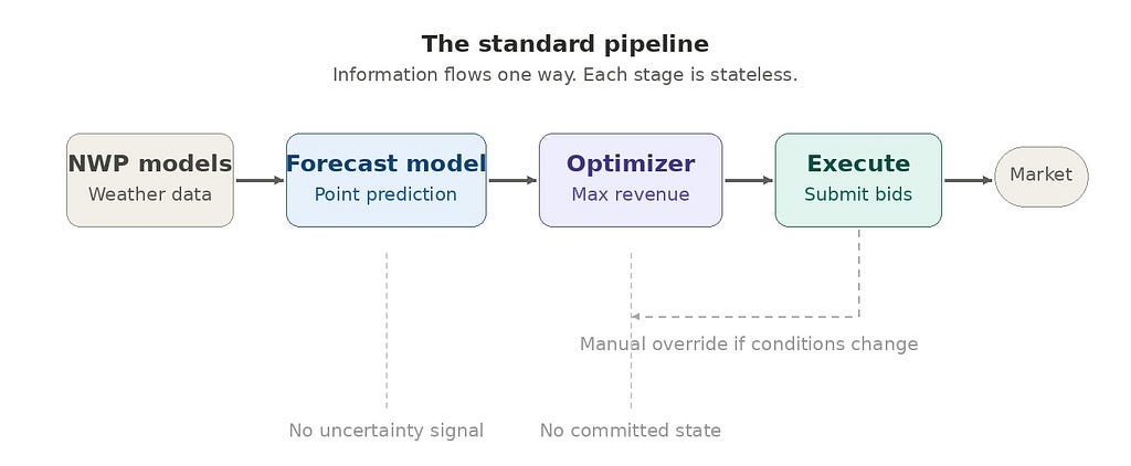
Information flows left to right. Each component is stateless with respect to the others. Re-running the pipeline means restarting from the beginning.
Policy architecture:
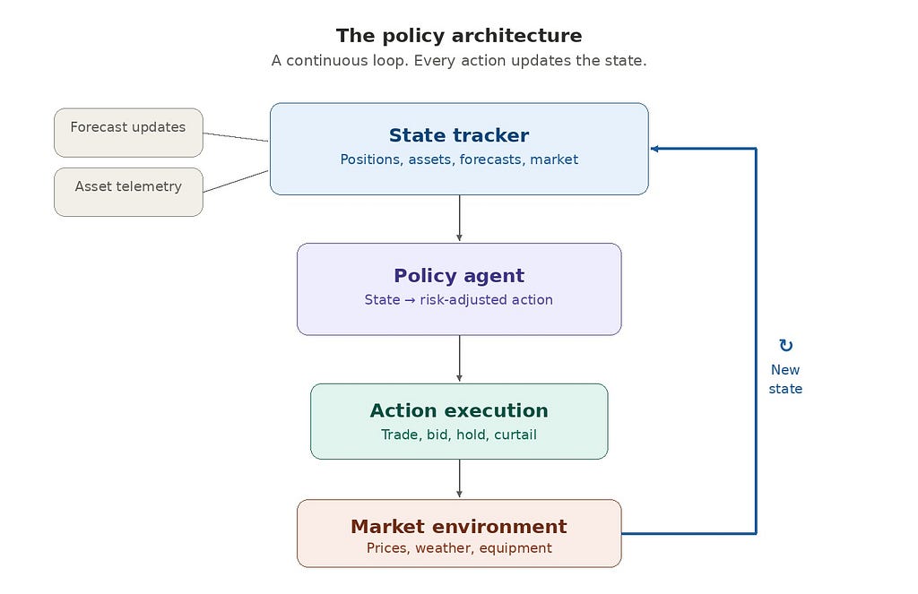
This is a loop, not a pipeline. Every action updates the state. Every state update feeds the next decision. The forecast is still there — it’s a critical input to the state tracker — but it no longer drives the architecture. The decision loop does.
If you’ve worked with agentic AI systems in other domains, this should look familiar. The observe-reason-act loop. The key differences in energy markets are: the environment is a regulated market with physical assets, the actions are financially binding, and the state space includes MWh, €/MWh, and MW of committed capacity alongside probabilistic forecasts and grid constraints.
Where the Policy Comes From
A natural question: where does the policy mapping itself come from? How do you build the function that takes a high-dimensional state and returns the right action?
There are three families of approaches, each with different trade-offs in energy trading.
Stochastic programming. Model the problem as a multi-stage optimization under uncertainty. Generate scenario trees from your forecast ensemble and solve for the decision at each node that maximizes expected value (or a risk-adjusted variant). This is well-established in power systems [2][3] and has the advantage of being interpretable — you can trace why a particular action was chosen. The disadvantage is computational: the scenario tree grows exponentially with the number of stages and uncertainties.
Reinforcement learning. Train an agent through simulation. Build a market simulator that captures the essential dynamics — price processes, forecast errors, asset constraints, gate closure rules — and let the agent learn a policy through trial and error. The advantage is that RL can handle high-dimensional state spaces and discover non-obvious strategies [4][5]. The disadvantages are real: sample efficiency, the sim-to-real gap, and a chicken-and-egg problem — building a faithful simulator requires deep market modeling expertise and historical data that many organizations are still assembling. Electricity markets have features (regulatory interventions, market coupling, liquidity effects) that are particularly hard to simulate.
Hybrid approaches. Use stochastic programming for the coarse structure — the day-ahead position, the broad storage strategy — and RL or heuristic policies for the fine-grained intraday and balancing decisions where the action space is too large for exact optimization. This is where the most promising work appears to be heading, because it combines the interpretability of mathematical programming with the adaptability of learned policies.
Stochastic programming is well-established in production trading systems across European power markets. RL-based approaches are in earlier stages — pilot deployments and active research — but advancing quickly. The practical question for all three families is less “does this work in theory?” and more “what does it take to make it robust in production, under regulatory and market integrity constraints?”
The Forecast Doesn’t Disappear — It Transforms
A common misunderstanding: if the system is policy-based, does the forecast become irrelevant?
No. The forecast becomes more important — but its role changes.

In a pipeline, the forecast produces a point estimate that the optimizer consumes. Forecast quality is measured by MAE, RMSE, or similar accuracy metrics. A better forecast feeds a better schedule, and the relationship is roughly linear.
In a policy architecture, the forecast provides a distribution — and the shape of that distribution directly affects the policy’s behavior. Two days with the same mean forecast but different uncertainty profiles should produce different actions. A tight distribution suggests committing early and capturing spread. A wide distribution suggests holding flexibility, keeping storage available, and trading smaller volumes across multiple stages.
This means the forecasting challenge shifts. Calibration matters more than point accuracy. Ensemble consistency matters. The ability to produce reliable probabilistic forecasts — not just a mean and some error bars, but a genuine representation of the joint distribution across hours, assets, and locations — becomes the foundation the policy stands on.
In markets with significant intraday volatility, a well-calibrated probabilistic forecast fed to even a basic policy can outperform a world-class point forecast fed to a perfect optimizer. The reason is structural: the optimizer can only act on what it sees — and a point forecast hides exactly the information the policy needs most.
What Changes in Practice
If you’re running a forecast pipeline today and this argument is persuasive, what actually changes? The transition doesn’t happen overnight, and it doesn’t require throwing everything away.

Step 1: Add state tracking. Before building a policy, you need to know the state. Most trading desks track positions, but often in spreadsheets or disconnected systems. The first concrete step is a unified state tracker that ingests committed positions, asset telemetry, forecast updates, and market data into a single representation — updated continuously, not at forecast cycle intervals.
Step 2: Make the optimizer state-aware. Your existing optimizer can become the first crude policy. Instead of re-optimizing from scratch each cycle, condition it on the current state: what’s already committed, what’s still flexible, how much capacity remains. This alone eliminates the manual reconciliation problem.
Step 3: Introduce uncertainty-aware dispatch. Use your probabilistic forecast (even a simple ensemble) to evaluate actions against multiple scenarios rather than just the mean. When uncertainty is high, the system should prefer flexible actions. When it’s low, commit aggressively. This can be implemented as a scenario-weighted extension of your existing optimizer.
Step 4: Close the loop. Feed outcomes back into the state tracker. Every trade execution, every price realization, every forecast error becomes data that updates the state. The system stops being a pipeline that runs periodically and becomes a loop that runs continuously.
Step 5: Learn and improve the policy. Once the loop is running and generating data, you can begin optimizing the policy itself — through offline simulation, counterfactual analysis, or, eventually, online learning with appropriate safeguards. This step also intersects with regulatory requirements: automated trading systems in European electricity markets operate under REMIT [6] and must meet transparency and market integrity obligations. Policy governance — how you validate, audit, and approve changes to an autonomous decision system — becomes as important as the policy itself.
Each step is incremental. Each delivers value independently. But the cumulative effect is a system that behaves fundamentally differently from where it started.
The Revenue Gap Is a Decision Gap
The first post in this series argued that electricity markets are sequential decision systems. This post makes the next claim: the performance gap in renewable and hybrid portfolios is primarily a decision architecture gap, not a forecasting gap.
Improving your forecast from 8% MAE to 6% MAE matters. But if that better forecast still feeds a stateless optimizer that ignores committed positions, treats uncertainty as a nuisance, and evaluates each market stage independently — the improvement captures a fraction of its potential value.
The same forecast, feeding a state-aware policy that reasons across market stages, values flexibility, and adapts to conditions as they evolve — that captures the rest.
The energy transition is deploying enormous volumes of variable renewables and storage. The tools that manage these assets need to match the complexity of the markets they operate in. Forecasting is a maturing discipline — mature methods exist, and marginal accuracy gains are increasingly expensive. Decision architecture, by contrast, is an open problem — and the marginal gains available are large.
Next in the series: “Forecast Uncertainty as a Trading Signal: Beyond Point Predictions” — how ensemble spread, calibration, and distributional forecasts become direct inputs to trading decisions, not just error metrics.
This post is part of a series: AI Systems Architecture for Multi-Stage Electricity Markets.
References
[1] Kraft, E., Russo, M., Keles, D., & Bertsch, V. (2022). Stochastic optimization of trading strategies in sequential electricity markets. European Journal of Operational Research, 303(3), 1400–1412.
[2] Wozabal, D. & Rameseder, G. (2020). Optimal bidding of a virtual power plant on the Spanish day-ahead and intraday market for electricity. European Journal of Operational Research, 280(2), 639–655.
[3] Shinde, P., Kouveliotis-Lysikatos, I., & Amelin, M. (2022). Multistage Stochastic Programming for VPP Trading in Continuous Intraday Electricity Markets. IEEE Transactions on Sustainable Energy, 13(3), 1675–1686.
[4] Boukas, I., Ernst, D., & Papavasiliou, A. (2021). A deep reinforcement learning framework for continuous intraday market bidding. Machine Learning, 110, 2335–2387.
[5] Bertrand, G. & Papavasiliou, A. (2020). Adaptive trading in continuous intraday electricity markets for a storage unit. IEEE Transactions on Power Systems, 35(3), 2339–2350.
[6] Regulation (EU) 2024/1106 of the European Parliament and of the Council (REMIT II), amending Regulation (EU) No 1227/2011. Official Journal of the European Union, May 2024.
From Forecast Models to Policy Agents: Rethinking AI in Power Markets was originally published in Towards AI on Medium, where people are continuing the conversation by highlighting and responding to this story.