
You have spent three weeks tuning hyperparameters, experimenting with the latest transformer architecture, and building a slick training pipeline. Your model is finally converging. But when you run inference on real data, the predictions are off in ways that do not make sense. False positives cluster around edge cases you never considered. Certain classes are systematically misclassified. The validation accuracy looked great, yet the model fails where it matters most.
If this sounds familiar, the problem is probably not your learning rate schedule or your choice of optimizer. It is your labels.
Every supervised model in production today — from sentiment classifiers to self-driving car perception stacks — was trained on data that a human, or some combination of humans and tools, sat down and labelled.
The quality of those labels sets a hard ceiling on what your model can ever learn. A state-of-the-art architecture trained on noisy annotations will consistently underperform a simpler model trained on clean ground truth. The research has proven this again and again, yet most teams still treat labelling as a preprocessing chore rather than a first-class engineering task.
In this article, I will walk you through what data labelling actually involves, why it is the single biggest lever on model performance, and how to build labelling pipelines that produce ground truth you can trust.
What Is Data Labelling?
Data labelling (also called data annotation) is the process of adding meaningful tags, categories, or structured metadata to raw data so that machine learning models can learn from it. It is the bridge between raw, unstructured data and the supervised learning algorithms that power modern AI systems.
Without labelled data, supervised learning simply cannot exist. Every image classifier, sentiment model, named entity recognizer, and object detector in production was trained on annotated examples. The labels tell the model what to predict, and they implicitly define the decision boundaries the model will learn.
What makes labelling challenging is that it is not just about assigning tags. It is about designing a schema that is mutually exclusive, collectively exhaustive, and operationally definable. It is about handling edge cases consistently. It is about measuring whether different annotators agree on the same answer. And it is about doing all of this at scale without letting quality degrade.
Why Label Quality Beats Model Complexity
It is tempting to focus on architecture, hyperparameters, and training pipelines. But in practice, data quality is the single biggest lever on model performance. Research across the industry has consistently shown that:
- A state-of-the-art model trained on noisy labels will underperform a simpler model trained on clean labels.
- Mislabelled data introduces irreducible error — a ceiling that no amount of regularization or fine-tuning can break through.
- The cost of fixing label errors compounds downstream: a bad label in training can mean a bad prediction in production, and a bad prediction can mean a bad business decision.
Consider this scenario. You are building a medical image classifier to detect skin lesions. A few training images are mislabelled where a benign mole marked as malignant. Your model memorizes those patterns and starts flagging healthy skin as dangerous. The false positive rate rises. Clinicians lose trust. The project stalls. All because of a handful of incorrect labels that could have been caught with proper quality control.
The takeaway is simple: before you optimize your model, optimize your ground truth.
The Data Labelling Workflow
Regardless of domain or data type, most labelling pipelines follow a common structure. Understanding this flow helps you identify where quality typically breaks down.

- Raw Data Collection
Gather the un-labelled data you need. This could be text documents, images, audio clips, or sensor readings. At this stage, you also need to think about class balance and representation. If your production data contains rare edge cases but your labelled set does not, your model will fail on those cases.
2. Label Schema Design
Define what categories exist, what granularity you need, and how edge cases should be handled. This is the most cost-effective investment in any ML project. Changing the schema mid-annotation means re-labelling everything.
3. Annotator Assignment
Decide who labels the data. Options include subject-matter experts, trained in-house teams, crowdsourcing platforms, or automated tools. The right choice depends on task complexity, domain expertise required, and budget.
4. Annotation
The actual labelling work. This is where consistency either holds or breaks. Clear guidelines, worked examples, and regular calibration sessions are essential.
5. Quality Control & Review
Measure inter-annotator agreement, run expert reviews, and flag inconsistencies. This step catches the errors that would otherwise become training noise.
6. Label Consolidation
Merge labels from multiple annotators, resolve conflicts through majority vote or adjudication, and produce the final ground truth dataset.
7. Active Learning Loop (Optional)
Train an initial model, have it flag uncertain samples, send those back to human reviewers, and iterate. This can reduce labelling costs by 50–80% while maintaining accuracy.
Label Types: From Text to Pixels
Different tasks demand different label formats. Here is a quick reference for the most common types across NLP and computer vision.
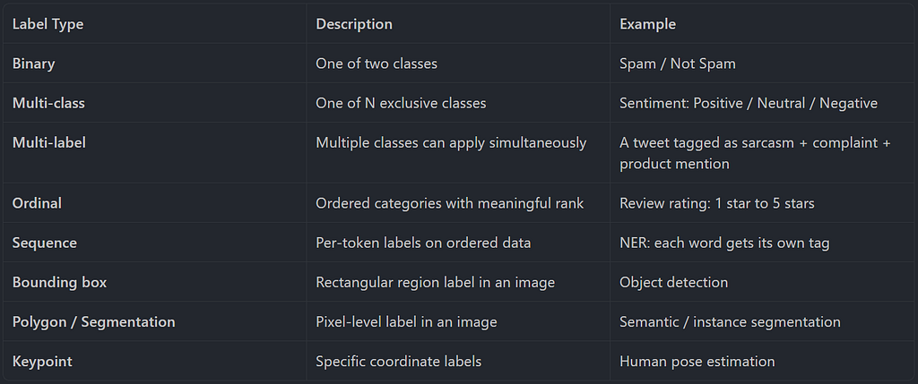
The task determines the label format, and the label format determines your annotation tool, your quality metrics, and your model architecture. Choose carefully.
NLP Labelling: Tokens, Entities, and Relations
Natural Language Processing tasks require labelling text ranging from assigning a single category to an entire document, down to tagging individual tokens within a sentence.
Text Classification
The simplest form of NLP labelling. A human reads a piece of text and assigns it to one or more predefined categories. Sentiment analysis, topic classification, intent detection, and toxicity detection all fall into this category.
The challenge is not the format. It is the ambiguity. Consider the review: “Great product but terrible shipping.” Is that positive, negative, or mixed? If three annotators label it differently, your model will learn conflicting signals. The fix is explicit handling rules in your annotation guideline, written before a single sample is tagged.
Named Entity Recognition and the BIO Scheme
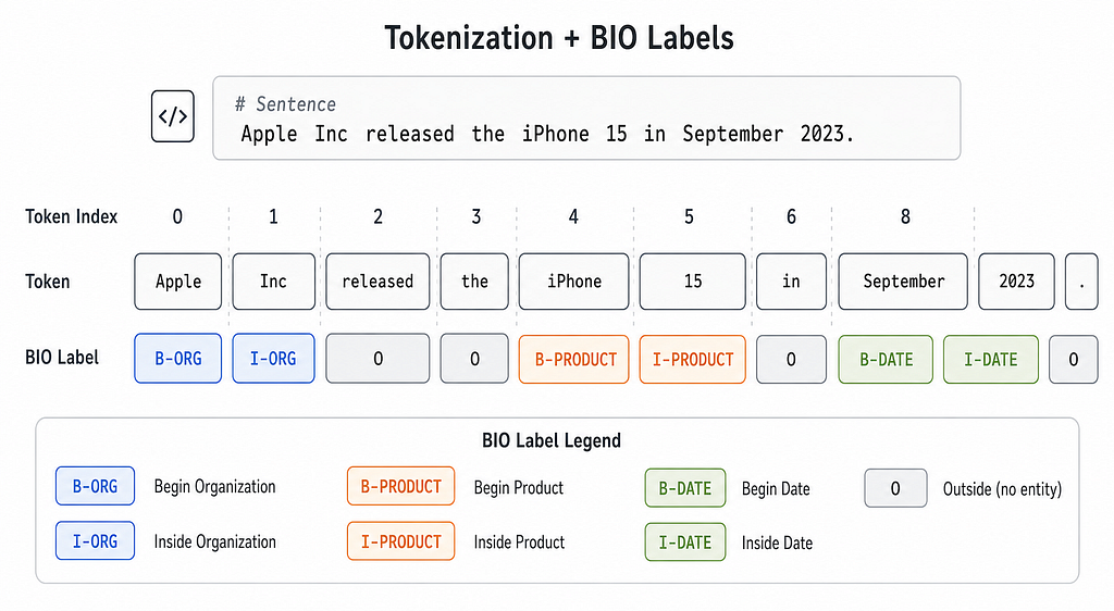
NER labelling assigns a tag to every token, identifying spans of text that refer to specific entity types. The industry-standard format is BIO tagging:
- B marks the beginning of an entity.
- I marks the inside of an entity.
- O means outside any entity.
Relation Extraction and Span Labelling
Relation extraction goes beyond NER to label the semantic relationship between entities. For example, in “Elon Musk founded SpaceX in 2002,” the relation FOUNDED_BY connects SpaceX (subject) to Elon Musk (object).
Question answering tasks use span labelling: given a context and a question, the annotator highlights the exact character span that answers it. These advanced tasks demand higher inter-annotator agreement because ambiguity is naturally higher.
Computer Vision Labelling: Boxes, Masks, and Keypoints

Computer vision labelling deals with images and video — requiring annotators to precisely mark spatial regions, boundaries, or points that correspond to objects or features of interest.
Object Detection and Bounding Box Formats
Object detection requires drawing rectangular bounding boxes around every target object and assigning each box a class label. But here is a trap that catches even experienced engineers: different frameworks expect different coordinate formats.
| Format     | Representation                                       | Used By                  |
| ---------- | ---------------------------------------------------- | ------------------------ |
| COCO       | `[x_min, y_min, width, height]`                      | COCO dataset, Detectron2 |
| Pascal VOC | `[x_min, y_min, x_max, y_max]`                       | Traditional CV pipelines |
| YOLO       | `[x_center, y_center, width, height]` normalized 0-1 | YOLO family models       |
Forgetting which format your data loader expects will silently corrupt every label in your dataset. Always verify your format before training. Here is an example code snippet than you can run:
"""
Bounding Box Format Conversion

This script converts between the three most common bounding box formats
used in computer vision: COCO, Pascal VOC, and YOLO.

Forgetting which format your data loader expects will silently corrupt
every label in your dataset. Always verify before training.
"""


def coco_to_yolo(bbox, img_width, img_height):
    """
    Convert COCO [x_min, y_min, width, height] to YOLO [x_c, y_c, w, h] normalized.

    Args:
        bbox: List [x_min, y_min, width, height] in absolute pixels
        img_width: Width of the image in pixels
        img_height: Height of the image in pixels

    Returns:
        List [x_center, y_center, width, height] normalized to 0-1
    """
    x_min, y_min, w, h = bbox
    x_center = (x_min + w / 2) / img_width
    y_center = (y_min + h / 2) / img_height
    w_norm = w / img_width
    h_norm = h / img_height
    return [x_center, y_center, w_norm, h_norm]


def yolo_to_pascal_voc(bbox, img_width, img_height):
    """
    Convert YOLO [x_c, y_c, w, h] normalized to Pascal VOC [x_min, y_min, x_max, y_max].

    Args:
        bbox: List [x_center, y_center, width, height] normalized to 0-1
        img_width: Width of the image in pixels
        img_height: Height of the image in pixels

    Returns:
        List [x_min, y_min, x_max, y_max] in absolute pixels
    """
    x_c, y_c, w, h = bbox
    x_min = int((x_c - w / 2) * img_width)
    y_min = int((y_c - h / 2) * img_height)
    x_max = int((x_c + w / 2) * img_width)
    y_max = int((y_c + h / 2) * img_height)
    return [x_min, y_min, x_max, y_max]


def pascal_voc_to_coco(bbox):
    """
    Convert Pascal VOC [x_min, y_min, x_max, y_max] to COCO [x_min, y_min, width, height].

    Args:
        bbox: List [x_min, y_min, x_max, y_max] in absolute pixels

    Returns:
        List [x_min, y_min, width, height] in absolute pixels
    """
    x_min, y_min, x_max, y_max = bbox
    w = x_max - x_min
    h = y_max - y_min
    return [x_min, y_min, w, h]


if __name__ == "__main__":
    # Example: 640x480 image with a COCO-format bounding box
    img_w, img_h = 640, 480
    coco_bbox = [120, 85, 200, 150]  # [x_min, y_min, width, height]

    print(f"Original COCO:     {coco_bbox}")

    # COCO -> YOLO
    yolo_bbox = coco_to_yolo(coco_bbox, img_w, img_h)
    print(f"Converted YOLO:    {[round(v, 4) for v in yolo_bbox]}")

    # YOLO -> Pascal VOC
    voc_bbox = yolo_to_pascal_voc(yolo_bbox, img_w, img_h)
    print(f"Converted VOC:     {voc_bbox}")

    # Pascal VOC -> COCO (round-trip verification)
    back_to_coco = pascal_voc_to_coco(voc_bbox)
    print(f"Back to COCO:      {back_to_coco}")

    # Verify round-trip consistency
    assert back_to_coco == coco_bbox, "Round-trip conversion failed!"
    print("\nRound-trip conversion successful. Your formats are consistent.")
Segmentation: Semantic vs Instance
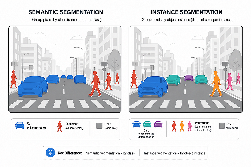
Semantic segmentation assigns a class label to every pixel, but does not distinguish between individual objects of the same class. Instance segmentation goes further by giving each object its own unique mask.
Keypoints and Pose Estimation
When shape matters more than boundaries, annotators label specific named coordinate points. The COCO 17-keypoint schema covers the human body from nose to ankle. Each keypoint carries a visibility flag: not labeled, occluded, or visible. This format powers pose estimation, facial landmark detection, and hand gesture recognition.
Measuring Label Quality
Before trusting any labelled dataset, you need objective quality metrics. The two most important are inter-annotator agreement and label error rate.
Inter-Annotator Agreement
Inter-annotator agreement measures how consistently different annotators label the same data. It is a fundamental proxy for label quality because if humans cannot agree, a model cannot reliably learn.
Cohen’s Kappa is the gold standard for two annotators because it corrects for chance agreement.
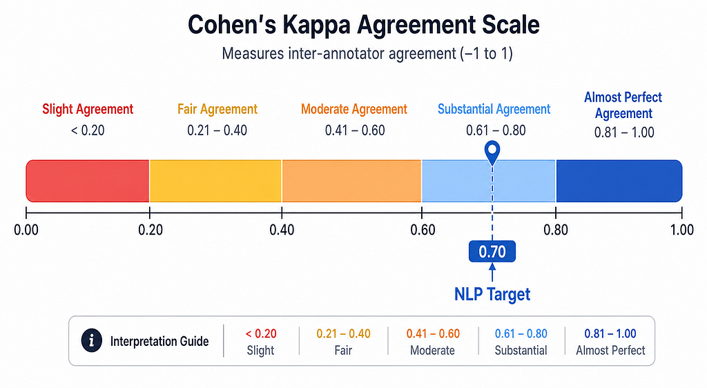
For most production NLP tasks, aim for a Kappa of at least 0.70. For medical or safety-critical computer vision tasks, 0.80 is the standard. Run a calibration round on 50–100 samples before scaling to your full dataset. Here is an example code snippets that you can run for demonstration:
"""
Cohen's Kappa: Measuring Inter-Annotator Agreement

This script demonstrates how to calculate Cohen's Kappa score
to measure agreement between two human annotators.
"""

from sklearn.metrics import cohen_kappa_score

# Example labels from two annotators on the same 10 samples
# 1 = positive class, 0 = negative class
annotator_1 = [1, 0, 1, 1, 0, 1, 0, 0, 1, 1]
annotator_2 = [1, 0, 1, 0, 0, 1, 1, 0, 1, 1]

# Calculate Cohen's Kappa (corrects for chance agreement)
kappa = cohen_kappa_score(annotator_1, annotator_2)
print(f"Cohen's Kappa: {kappa:.3f}")

# Interpretation guide
if kappa < 0.00:
    level = "Less than chance"
elif kappa <= 0.20:
    level = "Slight"
elif kappa <= 0.40:
    level = "Fair"
elif kappa <= 0.60:
    level = "Moderate"
elif kappa <= 0.80:
    level = "Substantial"
else:
    level = "Almost perfect"

print(f"Agreement Level: {level}")

# For production NLP tasks, aim for kappa >= 0.70
# For medical or safety-critical tasks, aim for kappa >= 0.80
print(f"\nProduction-ready? {'Yes' if kappa >= 0.70 else 'No - run another calibration round'}")
Label Error Rate
Even with high agreement, some labels will still be wrong. Tools like Cleanlab can detect likely label errors in a trained classifier by comparing model confidence against the assigned label.
If your estimated label error rate exceeds 3%, pause and audit before training your final model. Those errors are not just noise — they are training signals your model will memorize.
Smarter Ways to Label: Active Learning and Weak Supervision
Labelling everything manually is expensive and slow. Two strategies can dramatically reduce cost without sacrificing quality.
Active Learning
Instead of labelling all data randomly, train a model on a small seed set, then selectively label only the samples the model is most uncertain about. This focuses human effort where it matters most.
Uncertainty sampling strategies include:
- Least confidence: label samples where the top predicted probability is lowest.
- Margin sampling: label samples where the gap between the top two predictions is smallest.
- Entropy sampling: label samples with the highest prediction entropy across all classes.
Try running this code snippets to check the demonstration:
"""
Active Learning with Uncertainty Sampling

This script demonstrates a basic active learning loop using modAL.
Instead of labelling all data randomly, we train a model on a small seed set,
then selectively label only the samples the model is most uncertain about.

This can reduce labelling volume by 50-80% while maintaining accuracy.
"""

import numpy as np
from sklearn.ensemble import RandomForestClassifier

# Note: install modAL with: pip install modAL
from modAL.models import ActiveLearner
from modAL.uncertainty import uncertainty_sampling

# For this demo, we'll use synthetic data
# In practice, X_unlabelled would be your pool of unlabelled samples
from sklearn.datasets import make_classification
from sklearn.model_selection import train_test_split

# Generate synthetic dataset
X, y = make_classification(n_samples=1000, n_features=20, n_classes=2, random_state=42)

# Split into initial labelled set, unlabelled pool, and test set
X_initial, X_unlabelled, y_initial, y_unlabelled = train_test_split(
    X, y, train_size=50, random_state=42
)
X_pool, X_test, y_pool, y_test = train_test_split(
    X_unlabelled, y_unlabelled, test_size=0.3, random_state=42
)

# Initialize the active learner with a small labelled seed set
learner = ActiveLearner(
    estimator=RandomForestClassifier(random_state=42),
    query_strategy=uncertainty_sampling,
    X_training=X_initial,
    y_training=y_initial
)

print(f"Initial accuracy on test set: {learner.score(X_test, y_test):.3f}")

# Active learning loop: query the most uncertain samples for human labelling
n_queries = 20
for iteration in range(n_queries):
    # The model tells us which sample it is most uncertain about
    query_idx, query_instance = learner.query(X_pool)

    # In a real workflow, you would present this sample to a human annotator
    # Here we simulate the human label using our held-out ground truth
    y_new = y_pool[query_idx].reshape(1,)

    # Teach the model the new label
    learner.teach(X_pool[query_idx], y_new)

    # Remove the labelled sample from the pool
    X_pool = np.delete(X_pool, query_idx, axis=0)
    y_pool = np.delete(y_pool, query_idx, axis=0)

    acc = learner.score(X_test, y_test)
    print(f"Iteration {iteration + 1:2d} | Pool size: {len(X_pool):4d} | Accuracy: {acc:.3f}")

print("\nKey principle: The model guides human effort to where it matters most.")
print("Never use active learning for your evaluation set -- keep that fully human-annotated.")
Weak Supervision
Weak supervision uses programmatic labelling functions from simple heuristics, keyword rules, or existing models, to generate noisy labels at scale. The Snorkel framework pioneered this approach.
Below is the code demostration of this concept:
"""
Weak Supervision with Snorkel

This script demonstrates how to use programmatic labelling functions
(keyword rules, heuristics, patterns) to generate noisy labels at scale.

The labels are then combined using a generative model to produce
probabilistic training labels for a downstream classifier.

Use this when you have massive unlabelled data and limited annotation budget.
Never use weak supervision labels for your evaluation ground truth.
"""

import pandas as pd
import numpy as np

# Note: install snorkel with: pip install snorkel
from snorkel.labeling import labeling_function, PandasLFApplier, LFAnalysis
from snorkel.labeling.model import LabelModel

# Define label constants
POSITIVE = 1
NEGATIVE = 0
ABSTAIN = -1


# --- Labelling Functions ---
# Each LF is a simple heuristic that votes on a label or abstains

@labeling_function()
def lf_contains_positive_word(x):
    """Vote POSITIVE if text contains strong positive words."""
    positive_words = ["great", "excellent", "love", "amazing", "perfect", "fantastic"]
    return POSITIVE if any(w in x.text.lower() for w in positive_words) else ABSTAIN


@labeling_function()
def lf_contains_negative_word(x):
    """Vote NEGATIVE if text contains strong negative words."""
    negative_words = ["terrible", "awful", "hate", "broken", "worst", "horrible"]
    return NEGATIVE if any(w in x.text.lower() for w in negative_words) else ABSTAIN


@labeling_function()
def lf_contains_exclamation_positive(x):
    """Vote POSITIVE if text has exclamation mark and positive sentiment words."""
    positive_words = ["great", "love", "amazing", "awesome"]
    has_positive = any(w in x.text.lower() for w in positive_words)
    has_exclaim = "!" in x.text
    return POSITIVE if (has_positive and has_exclaim) else ABSTAIN


@labeling_function()
def lf_contains_refund(x):
    """Vote NEGATIVE if text mentions refund or return."""
    return NEGATIVE if any(w in x.text.lower() for w in ["refund", "return", "money back"]) else ABSTAIN


# --- Create synthetic unlabelled data ---
data = {
    "text": [
        "This product is great! I love it.",
        "Terrible experience, would not recommend.",
        "Amazing quality for the price.",
        "Broken on arrival. Requesting refund.",
        "It is okay, nothing special.",
        "Absolutely perfect, exceeded expectations!",
        "Awful customer service, worst ever.",
        "Great value and fast shipping.",
        "Hate this product, complete waste.",
        "Not bad, but could be better."
    ]
}
df_unlabelled = pd.DataFrame(data)

# Apply all labelling functions to the unlabelled dataset
lfs = [
    lf_contains_positive_word,
    lf_contains_negative_word,
    lf_contains_exclamation_positive,
    lf_contains_refund
]

applier = PandasLFApplier(lfs=lfs)
L_train = applier.apply(df=df_unlabelled)

# Analyze LF coverage, overlap, and conflict
print("Labelling Function Analysis:")
print(LFAnalysis(L=L_train, lfs=lfs).lf_summary())
print()

# Train a generative label model to combine LF outputs into probabilistic labels
# The model learns to weight each LF based on its accuracy and correlation
label_model = LabelModel(cardinality=2, verbose=True)
label_model.fit(L_train=L_train, n_epochs=500, lr=0.001, seed=42)

# Predict probabilistic labels for the training set
y_prob = label_model.predict_proba(L=L_train)
y_pred = label_model.predict(L=L_train)

print("Weak supervision labels (0=Negative, 1=Positive):")
for text, pred, prob in zip(df_unlabelled["text"], y_pred, y_prob):
    confidence = prob[pred] if pred in [0, 1] else 0.5
    print(f"  [{pred}] (confidence: {confidence:.2f}) {text}")

print("\nRemember: these labels are noisy. Use them to train a downstream model,")
print("but never use them as ground truth for evaluation.")
Designing a Label Schema That Lasts
Getting the schema right before annotation starts is the highest-leverage decision in any labelling project. Changing it mid-annotation means relabelling everything that came before.
A good label schema follows four principles:
- Mutually Exclusive (for single-label tasks)
Every sample should unambiguously fall into exactly one category. If annotators frequently debate which label applies, the schema needs refinement.
2. Collectively Exhaustive
Every sample must have a valid label. An “Other” category is acceptable, but if it captures more than 10% of your data, the schema is underspecified.
3. Operationally Definable
Every label must be definable in terms of observable characteristics, not internal states or intentions that vary by annotator. “Sarcastic” is hard to define consistently. “Contains a positive word followed by a negative outcome” is more operational.
4. Task-Aligned
Labels should reflect what the downstream model actually needs to predict. Overly fine-grained labels that a model cannot meaningfully distinguish add cost without value.
Every production labelling project also needs a written annotation guideline covering the task definition, label definitions with examples, a decision tree for ambiguous cases, explicit exclusion rules, and quality standards including minimum IAA and review processes.
Common Labelling Challenges and Solutions

When Are Labels Good Enough?
Before you declare a dataset production-ready, run through this checklist:
- IAA (Cohen’s Kappa) is at least 0.70 for all label types.
- Label error rate is below 3%, estimated via Cleanlab or manual audit.
- Class distribution reflects expected production distribution.
- Edge cases and known failure modes are explicitly represented.
- Train, validation, and test splits are stratified with no label leakage.
- Annotation guidelines were reviewed and signed off by a domain expert.
- At least one round of annotator calibration was completed before full annotation.
- Evaluation set labels were reviewed by a senior annotator or expert, not just crowdsourced.
If any item on this list is missing, your dataset is not ready for production training. Fix it now. The cost only grows downstream.
Final Thoughts
Data labelling is not glamorous work. It does not get conference keynotes or GitHub stars. But it is the invisible foundation that every successful supervised learning system is built on. The best ML engineers I know spend more time on annotation guidelines and quality control than on architecture search.
The next time your model underperforms, ask yourself: when was the last time I looked at the labels? When was the last time I measured inter-annotator agreement? When was the last time I audited my evaluation set for errors?
Clean labels are the real competitive advantage. Architecture is shareable. Hyperparameter recipes are public. But a well-designed, rigorously validated labelled dataset is an asset that compounds in value over time.
Here are several key takeaways from this article:
- Label quality beats model complexity. A simple model on clean labels will outperform a complex model on noisy ones every time.
- Design your schema before touching a single sample. Changing labels mid-project means relabelling everything.
- Measure IAA before scaling. Run a calibration round on 50–100 samples and aim for Kappa >= 0.70.
- Know your bounding box formats. COCO, Pascal VOC, and YOLO use different coordinate representations — verify before training.
- Active learning is the most cost-efficient path. It can cut labelling volume by half while maintaining accuracy, but never use it for your test set.
- Weak supervision bootstraps training data. Use Snorkel-style labelling functions to generate noisy training labels at scale, but keep evaluation sets fully human-annotated.
- Your evaluation set is sacred. Never use auto-annotation or weak supervision for ground truth you plan to measure performance against.
Thank you for reading this article! I hope you found it helpful. If you have any questions or feedback, please feel free to reach out to me.
#MachineLearning #DataScience #AIEngineering #DataLabelling #ComputerVision #NLP #SupervisedLearning #MLOps #DataAnnotation
Data Labelling: The Foundation of Supervised Machine Learning was originally published in Towards AI on Medium, where people are continuing the conversation by highlighting and responding to this story.