In my past article I wrote about how I implemented Character Level Tokenization over a very small corpus and understood the most basic and initial phases of NLP and base of LLMs.
This time I implemented the next step towards Modern NLP and LLM system “Embeddings” and implemented it from scratch and trained it over my laptop which took 30+ hours.
Let’s dive into the concept, mathematics and code that i understood in my process of building LLM from scratch and implementing the embeddings to my corpus of nearly 1 million words.
What are Embeddings?
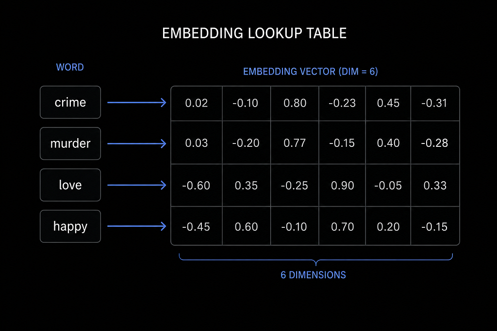
Embeddings are just the vector representation or format of each word to make the machine or model understand the word instead of making it memorize it with a unique number given to each unique words in a corpus.
For simple breakdown of concept of embeddings, let’s take an example:
Text = "dog cat"
dog = (0.01, 0.04, 0.2)
cat = (0.01, 0.03, 0.2)
# dog and cat are given similar vectors because they appear in similar context
So, now these two words can easily be represented in a 3D space in the form of vector, and these dense vectors allow neural networks to capture semantic relationships between words instead of treating every word as an isolated symbol to make them related to each other.
It transforms words into a format like:
king − man + woman ≈ queen
Not because anyone programmed it but semantic relationships emerged geometrically.
Those shocked researchers.

Why Early NLP Models Needed Embeddings ?
So, first and most important question “WHY”
Statistical language models only stored how frequently consecutive words appeared together.
They had no understanding of what those words actually meant.
So, if the Tokenizer model learns ‘dog barks’,
it learnt nothing about ‘cat meows’.
That’s just a single stated problem which is huge because without solving this, nothing could have been proceeded in AI world as context is the main concern till now.
But for more problems were like data sparsity as it knows only what has been trained or what was there in training dataset, if anything outside of that came to the model, it predicted very close to 0.
Explosion of memory as n increased in n-gram models.
Curse of One-Hot-Encodings:
If vocabulary size = 50,000:
1) Each word becomes 50,000-dimensional vectors.
2) Since one-hot vectors are orthogonal to each other, the model cannot naturally represent semantic similarity between related words like ‘dog’ and ‘cat’.
All these problems were needed to be solved to make the NLP applicable in real life.
Then came a major breakthrough in 2003 Bengio, Neural Language Models. where they used neural networks to learn dense vectors.
After Tokenizer and Before Embeddings
After implementing the tokenizer from scratch, what I had was a system that tokenizes each character from the corpus and predicts what should come next with the help of bigram and SoftMax function.
But now I had to increase the corpus size vastly and characters don't carry semantic meaning and character-level modeling also required much longer sequences and made semantic learning slower, which pushed me toward word-level representations.
Being a Dostoevsky devotee, I scraped his 5 novels which were:
1. The Brothers Karamazov
2. The Idiot
3. Short Stories by Dostoevsky
4. The Possessed (The Devils)
5. Notes From the Underground
These gave me a corpus of nearly 1Million words for training the embeddings.
How Do Embeddings Learn Meaning?
This all starts with corpus of text that we have and extracting the unique words from it to build the vocabulary.
Deciding dimensions of each vector.
Embedding dimensions are a hyperparameter and a rough starting point is the 4th root of your vocabulary size but that gives you just 15 dimensions for 50,000 words which is too small to capture anything meaningful. In practice 100–300 dimensions is what most implementations use. Higher dimensions capture more context but take longer to train and can overfit on smaller datasets.
In my case i used 32 because of hardware constraints, not because it was the ideal number.
Then moving forward, once the dimensions are decided, each word is initialized to a random vector which are later trained so that words appearing in similar contexts get closer in vector space.
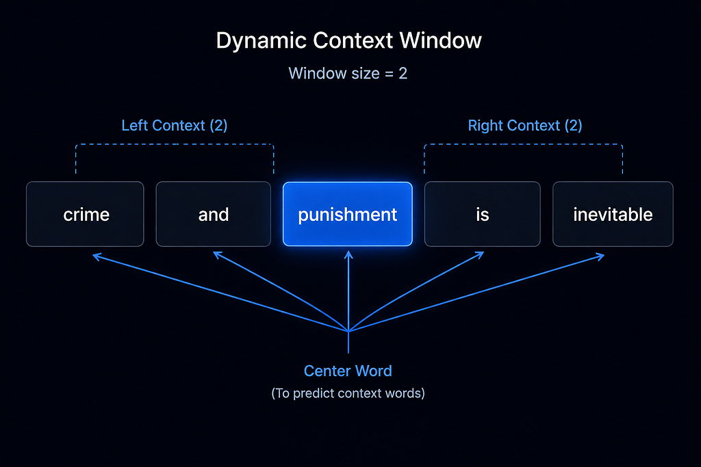
Context Window for each word
So, once the dimensions are fixed, we decide the max context size for each word and make two separate tables for context word’s embeddings and center word’s embeddings, the reason for two separate tables will be covered in the code section.
Negative Sampling
I added 5 fake samples for each real pair of context and center word by choosing the context word randomly for the same center word.
Something with no real relationship to the center word, like {Crime, Banana}.
Training the Embeddings
We pass these pairs for training where their untrained embeddings are fetched.
Dot products are taken to measure similarity and alignment.
score = np.dot(center_vec, context_vec)
If this score is high, the model thinks these words belong together. If low or negative, the model thinks they are unrelated.
Then the scores are passed through sigmoid function which makes them in the range of (0,1)
A very negative score maps close to 0, score = 0 becomes 0.5 and positive maps closer to 1.
Loss Function
The loss function penalizes the model when real word-context pairs receive low probabilities or when randomly sampled negative pairs receive high probabilities.
Losspositive = −log(σ(Vc ⋅ Vo)) # Model wants this probability close to 1.
Lossnegative = −log(1−σ(Vc ⋅ Vn)) # Model wants this probability close to 0.
Gradients
A gradient tells the model how much each number inside the vectors contributed to the prediction error and in which direction it should be adjusted to reduce the loss
Mathematically, gradients are the derivative of loss with respect to the score i.e. Prediction — Truth (this is only for sigmoid activation and binary cross entropy loss)
Backpropagation
It just understands error reduction and asks “Which number inside the vector caused the bad prediction”
i.e. How the gradients actually flow backwards to update and optimize the vectors.
How vectors actually change using learning rate is:
vector = vector - learning_rate * gradient
This is how actual learning happens, where vectors physically move in space.
Training Loop:
how many times we pass through the data and how loss changes over epochs. So, one epoch is basically going through this whole process over every pair of vectors for once.
Over multiple epochs Loss gradually decreases and the vector drifts towards the meaningful position in space.
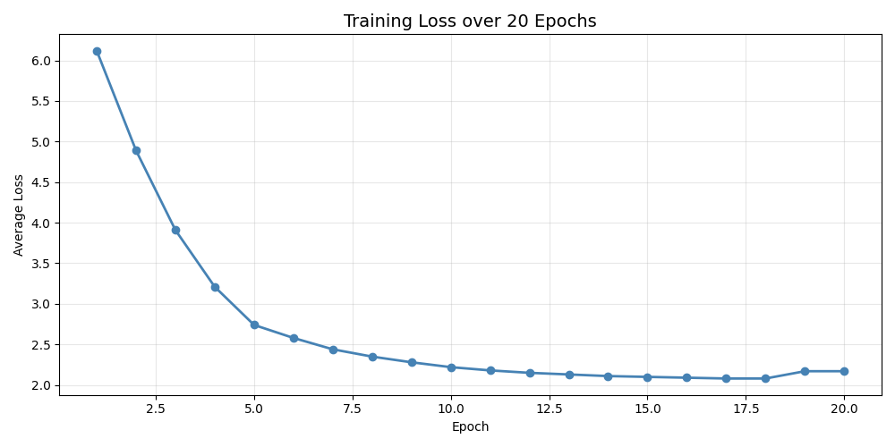
I trained the model for over 20 epochs and with 5 negative samples for each pair which took 30+ hours to train, and the results were actually remarkable.
I was not expecting many changes because in actual Google’s research paper where they trained the Skip-Gram model with negative sampling had a massive amount of data and trained for much longer time which was not even comparable with mine.
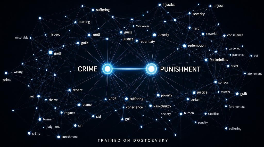
Below are the vector representations of words from the corpus, before and after training.
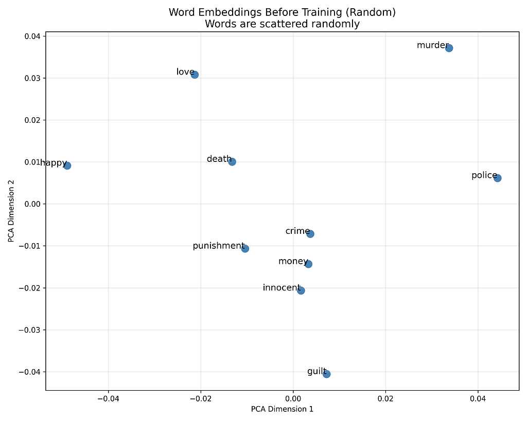
Just observe the vector of murder and crime how far they are before training which would change in the next image which is representation of vectors after training.
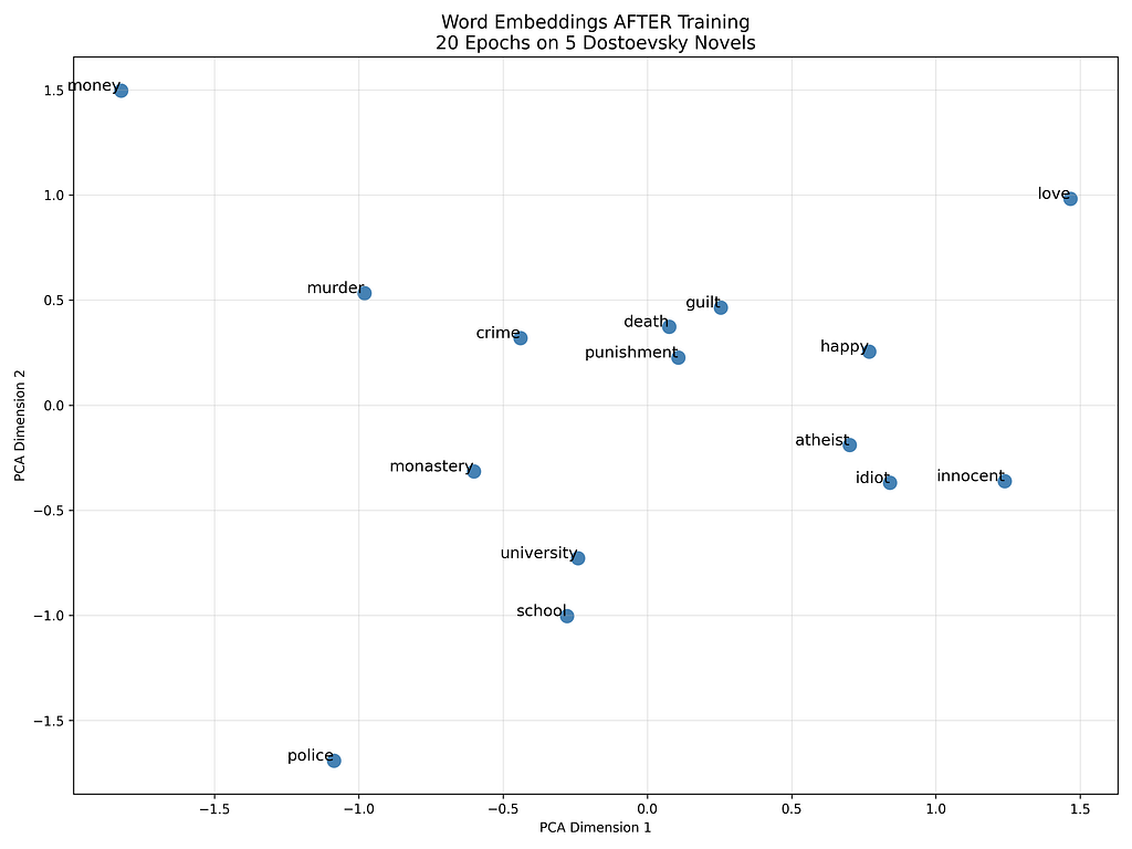
After 20 epochs: School, university, and monastery cluster together, and murder moves close to crime, punishment, and death
Why Skip-Gram not CBOW?
So, there are two popular architectures for training word embeddings, Skip-Gram and CBOW (Continuous Bag of Words) and they are essentially inverses of each other.
CBOW takes multiple context words and predicts the center word. Skip-Gram does the opposite; it takes one center word and predicts the surrounding context words.
The reason I went with Skip-Gram is simple, it generates far more training pairs. A single center word with a window of 2 produces 4 pairs and across 1 million words, that compounds into even more millions of training examples giving the model more chances to learn from every word.
This architecture was first introduced by Mikolov et al. in Efficient Estimation of Word Representations in Vector Space (2013), the paper that gave us Word2Vec.
Code Implementation
Let’s get into the actual code and I’ll only explain the parts that actually matter.
Processing:
text = text.lower()
text = re.sub(r'[^a-z\s]', '', text)
words = text.split()
Lowercasing everything and stripping punctuation so the model doesn’t treat “Crime” and “crime” as two different words.
Vocabulary and Tokenization:
word_to_idx = {w: i for i, w in enumerate(unique_words)}
tokens = [word_to_idx[w] for w in words]
Every unique word gets a number, and the entire corpus becomes a sequence of those numbers. This is what gets fed into training.
Two Embedding Tables:
input_embeddings = np.random.uniform(-0.5, 0.5, (vocab_size, embedding_dim)) / embedding_dim
output_embeddings = np.zeros((vocab_size, embedding_dim))
Why two embedding tables?
Looking closely, we can see that a single word plays 2 roles once as center embedding which is looked up in input_embeddings and when it acts as context word it is looked up in output_embeddings.
Initially I trained the model with a single embedding table which didn’t give good results. Love’s embedding closely aligned with crime’s embeddings which made no sense. Then i studied what was failing and found out that when same word plays both the role at different point in training, gradients from both roles collide and interfere with each other during backpropagation (with single table).
In simple words this made every word look similar. This was changed by two separate tables that kept the updates clean and isolated.
After training is done, input_embeddings is what you save and use. That is your final word representation.
Negative Sampling Distribution
word_freq = word_freq ** 0.75
This one line is actually important. Raw word frequency would make common words like “the” or “and” dominate the negative samples.
Raising frequency to the power of 0.75 smooths that out, giving rare words a fairer chance of being sampled as negatives. This comes directly from the original Word2Vec paper.
Training Loop
grad = prob - 1
input_embeddings[center_idx] -= learning_rate * grad * context_vec
output_embeddings[context_idx] -= learning_rate * grad * center_vec
This is where actual learning happens. The gradient for real pairs is
“Prob-1”and for negative pairs it is just “prob”, this is basically the derivative of binary cross entropy loss with sigmoid activation which I mentioned earlier. Every update physically moves the vectors in space, pulling related words closer and pushing unrelated ones apart.
Results after training
Results after training were impressive. I already showed the PCA representation before training. Below are the actual cosine distances between the vectors after 20 epochs.

Above image shows the actual cosine distances between the vectors with similar context like school was found similar with supper, university, monastery which are really good.
Distance between crime and punishment decreased drastically after training and same for crime and murder
Limitations
32 dimensions are actually too small to understand the context with higher accuracy.
Real Word2Vec used 300 dimensions and 20 epochs are also relatively very few, higher epochs would align the vectors more accurately.
As I trained the model over single author, it made these embeddings carry Dostoevsky’s worldview.
A general language model would look different from this.
I implemented this model purely over NumPy loops which are slow.
Real implementation used Batched Matrix Operation which took days for google even in such a large amount of dataset as they ran over thousands of machines.
Whereas mine took 30+ hours even with such a small dataset compared to actual implementation by google.
What I learned building this
Embeddings do not predict anything on their own. They just give words meaning before passing them into the model.
The pipeline so far:
Text → Tokenizer → Token IDs → Embeddings → [???] → Prediction
That gap in the middle is attention. That’s where the model actually figures out which words should influence each other in a sequence.
Where actual prediction begins.
That’s what I’m building next.

Vinayak this side.
Building an LLM from scratch, one step at a time.
Follow the full code on GitHub or connect with me on LinkedIn.
Building an LLM From Scratch: I Trained Word Embeddings on Dostoevsky. Here’s What I Found. was originally published in Towards AI on Medium, where people are continuing the conversation by highlighting and responding to this story.