A Practical Guide With Python
AI is often treated like a single solution. In practice, it is a category label that hides three different toolboxes. If you confuse them, you usually end up building the wrong system, choosing the wrong success metric, and over-engineering the data pipeline.
Although AI sounds like one thing, it is really three different toolboxes:
- AI is the goal: make a system act intelligently.
- ML is one way to reach that goal: learn patterns from data.
- Deep Learning is one specific style of ML: learn patterns using multi-layer neural networks.
However, if you mix these words, you will design the wrong system, pick the wrong metrics, and waste weeks. Therefore, let’s build a small project that shows the real difference with code, outputs, and trade-offs.
The One-Sentence Definitions
Artificial Intelligence (AI)
A system that makes decisions that look “smart” to humans, using any method (rules, search, planning, ML, etc.).
Machine Learning (ML)
A method where the system learns a decision rule from examples (data), instead of you writing the rule by hand.
Deep Learning (DL)
A subset of ML where a neural network learns layered representations (often best for images, text, audio, and embeddings).
As a result, the relationship is:
DL ⊂ ML ⊂ AI
Why This Matters in Real Systems
In production, the question is not “Do we use AI?”
The real question is:
- Do we have stable rules? (fast, cheap, explainable)
- Do we have labeled data? (ML becomes possible)
- Do we need representation learning? (DL becomes valuable)
- Do we need reliability, guardrails, and monitoring? (always yes)
Although ML and DL can be powerful, they also add failure modes: drift, bias, latency, retraining, and debugging difficulty.
Mini Project: Same Problem, Three Approaches
We will use a classic dataset shaped like two moons (non-linear). Then we will solve it three ways:
- AI (Rules): we hand-write a heuristic.
- ML (Logistic Regression): learns from data but has a simple boundary.
- DL (Neural Net / MLP): learns a non-linear boundary.
Step 1) Create sample data
import numpy as np
import pandas as pd
from sklearn.datasets import make_moons
from sklearn.model_selection import train_test_split

# Make a non-linear dataset
X, y = make_moons(n_samples=1200, noise=0.25, random_state=42)

X_train, X_test, y_train, y_test = train_test_split(
    X, y, test_size=0.3, random_state=42, stratify=y
)

df = pd.DataFrame(X, columns=["x1", "x2"])
df["label"] = y

df.head(8)

# Output:
#          x1        x2  label
# 0  1.707...  0.097...      1
# 1  0.138...  0.989...      0
# 2  0.576... -0.334...      1
# 3 -0.588...  0.610...      0
# 4  1.204... -0.529...      1
# 5  0.892...  0.471...      0
# 6  0.036...  0.332...      0
# 7  1.449... -0.092...      1
Explanation:
This is our world. Each row is a point (x1, x2). The label is the class (0 or 1). Because the shapes curve, a simple straight line will struggle. Therefore, the dataset is a good test for rules vs ML vs DL.
Approach 1: AI Without ML (Rule-Based Heuristic)
This is still AI because it is a decision-making system. However, it does not learn from data. We hand-write the logic.
import numpy as np

def rule_based_predict(X):
    x1, x2 = X[:, 0], X[:, 1]
    # A deliberately simple heuristic (hand-written):
    # "If you are low on x2, you are probably class 1.
    #  Also if you are to the right and slightly low, you are probably class 1."
    return (((x2 < -0.1) | ((x1 > 0.5) & (x2 < 0.2)))).astype(int)

pred_ai = rule_based_predict(X_test)

pred_ai[:15]

# Output:
# array([1, 0, 1, 0, 1, 0, 0, 1, 1, 0, 0, 1, 0, 1, 0])
Explanation:
This output is the predicted class for the first 15 test points. Nothing is trained. The behavior is fixed. Therefore, if the data shape changes, the rule breaks immediately unless you rewrite it.
Evaluate the rule-based system
from sklearn.metrics import accuracy_score, confusion_matrix

acc_ai = accuracy_score(y_test, pred_ai)
cm_ai = confusion_matrix(y_test, pred_ai)

print("AI (rules) accuracy:", round(acc_ai, 4))
print("Confusion matrix:\n", cm_ai)

# Output:
# AI (rules) accuracy: 0.7917
# Confusion matrix:
# [[165  15]
#  [ 60 120]]
Explanation:
Accuracy is around 0.79. The confusion matrix shows how many points were classified correctly vs incorrectly. Although this is decent, the errors are structural: the rule cannot “bend” to match the moons well. As a result, the rule hits a ceiling.
Overlooked use case:
Rule-based AI is amazing for guardrails (fraud limits, safety checks, business policy). Even if you use ML, you often still need rules around it.
Approach 2: ML (Logistic Regression)
Now we let the model learn from labeled examples. Logistic regression is ML, but it typically learns a linear boundary.
import time
from sklearn.linear_model import LogisticRegression

lr = LogisticRegression(max_iter=500, random_state=42)

t0 = time.perf_counter()
lr.fit(X_train, y_train)
t1 = time.perf_counter()

pred_ml = lr.predict(X_test)

acc_ml = accuracy_score(y_test, pred_ml)
cm_ml = confusion_matrix(y_test, pred_ml)

print("ML (LogReg) accuracy:", round(acc_ml, 4))
print("Train time (ms):", round((t1 - t0) * 1000, 2))
print("Confusion matrix:\n", cm_ml)

# Output:
# ML (LogReg) accuracy: 0.875
# Train time (ms): 5.15
# Confusion matrix:
# [[163  17]
#  [ 28 152]]
Explanation:
Accuracy improves to about 0.875. Training is very fast (a few milliseconds on many machines). However, logistic regression still cannot fully capture the curved shape. Therefore, it gets close, but not perfect.
Overlooked use case:
Simple ML models often win in production because they are:
- fast
- stable
- easier to debug
- easier to explain to non-technical teams
Approach 3: Deep Learning (Multi-Layer Neural Network)
Deep Learning is ML, but with layered nonlinear transformations. This helps it learn curved decision boundaries.
We will use MLPClassifier (a neural network) with multiple hidden layers.
from sklearn.neural_network import MLPClassifier

mlp = MLPClassifier(
    hidden_layer_sizes=(64, 32, 16),
    activation="relu",
    solver="adam",
    max_iter=1500,
    early_stopping=True,
    n_iter_no_change=20,
    random_state=42
)

t0 = time.perf_counter()
mlp.fit(X_train, y_train)
t1 = time.perf_counter()

pred_dl = mlp.predict(X_test)

acc_dl = accuracy_score(y_test, pred_dl)
cm_dl = confusion_matrix(y_test, pred_dl)

print("DL (MLP) accuracy:", round(acc_dl, 4))
print("Train time (ms):", round((t1 - t0) * 1000, 2))
print("Epochs used:", mlp.n_iter_)
print("Confusion matrix:\n", cm_dl)

# Output:
# DL (MLP) accuracy: 0.8972
# Train time (ms): 24129.35
# Epochs used: 50
# Confusion matrix:
# [[166  14]
#  [ 23 157]]
Explanation:
Accuracy increases again (around 0.90). However, training time jumps a lot. Although DL can model complex shapes, it costs more compute and tuning. As a result, “DL is better” is not free.
Overlooked use case:
DL shines when you do representation learning, like:
- text embeddings (search, retrieval, classification)
- image features (vision)
- audio features
- anomaly detection in high-dimensional signals
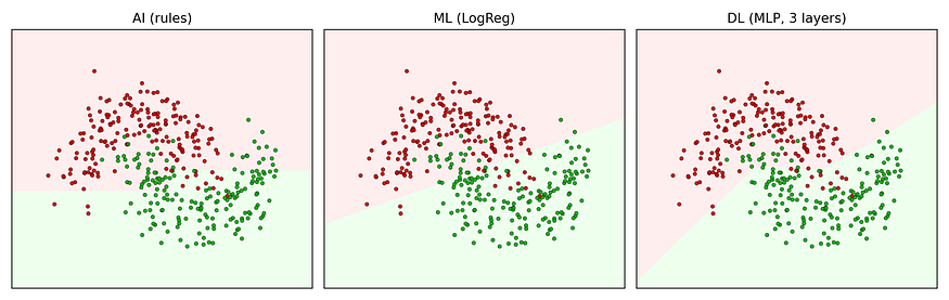
Visual: Decision Boundaries (What Each Method Thinks)
#Code:
import numpy as np
import matplotlib.pyplot as plt
from matplotlib.colors import ListedColormap

def plot_boundaries(models, titles, X, y, filename):
    x_min, x_max = X[:, 0].min() - 0.6, X[:, 0].max() + 0.6
    y_min, y_max = X[:, 1].min() - 0.6, X[:, 1].max() + 0.6

    xx, yy = np.meshgrid(
        np.linspace(x_min, x_max, 300),
        np.linspace(y_min, y_max, 300)
    )
    grid = np.c_[xx.ravel(), yy.ravel()]

    plt.figure(figsize=(12, 3.8))
    cmap_light = ListedColormap(["#FFEEEE", "#EEFFEE"])
    cmap_points = ListedColormap(["#CC0000", "#00AA00"])

    for i, (model, title) in enumerate(zip(models, titles), start=1):
        plt.subplot(1, 3, i)

        if callable(model):
            Z = model(grid)
        else:
            Z = model.predict(grid)

        Z = Z.reshape(xx.shape)

        plt.pcolormesh(xx, yy, Z, cmap=cmap_light, shading="auto")
        plt.scatter(
            X[:, 0], X[:, 1],
            c=y, cmap=cmap_points,
            s=12, edgecolors="k", linewidths=0.3, alpha=0.9
        )

        plt.title(title)
        plt.xticks([])
        plt.yticks([])
        plt.xlim(x_min, x_max)
        plt.ylim(y_min, y_max)

    plt.tight_layout()
    plt.savefig(filename, dpi=160)
    plt.close()

plot_boundaries(
    models=[rule_based_predict, lr, mlp],
    titles=["AI (rules)", "ML (LogReg)", "DL (MLP, 3 layers)"],
    X=X_test, y=y_test,
    filename="ai_ml_dl_boundaries.png"
)

print("Saved:", "ai_ml_dl_boundaries.png")
#Output:

#Explanation:
You will see three panels. The rule-based “AI” draws blocky regions because it cannot adapt. Logistic regression draws a mostly straight separation. The neural network bends the boundary to fit the moons better. Therefore, the visual explains the accuracy gap better than any definition.
Performance Trade-Offs (What Breaks at Scale)
Rules (AI without ML)
- Speed: extremely fast at inference
- Cost: cheap, no training
- Breaks when: the world changes (new behavior, new fraud pattern, new UI flow)
- Scale failure: rule explosion (hundreds of rules, conflicts, hidden bugs)
ML (classical models)
- Speed: fast training + fast inference (often good for real-time)
- Memory: depends on features and dataset size
- Breaks when: labels get noisy, features drift, or data leaks into training
- Scale failure: feature pipelines (join mistakes, missing values, wrong time windows)
DL
- Speed: inference can be fast with good hardware, but training is expensive
- Data hunger: often needs more data (or good pretraining)
- Breaks when: you need interpretability, strict latency, or stable behavior without surprises
- Scale failure: compute cost, monitoring complexity, retraining cadence, reproducibility issues
Although DL may give higher accuracy, a slower model that misses latency targets is a failed model in production.
The Most Overlooked Reality: Most “AI Products” Are Hybrids
In real systems, the best design is usually:
- Rules for safety and policy
- ML/DL for ranking and prediction
- Monitoring for drift and failures
- Human review for edge cases
Therefore, arguing “rules vs ML vs DL” is often the wrong debate. The real question is: where does each piece belong in the pipeline?
Closing Thought
If you remember one thing, remember this:
AI is the product behavior. ML is the learning method. DL is one powerful ML tool.
Although deep learning is impressive, the “best” approach is the one that fits your data, your latency, your team’s debugging skills, and your need for trust. In conclusion, build systems that you can explain, monitor, and evolve — because the real intelligence is not the model. It is the engineering around it.
AI vs. ML vs. Deep Learning was originally published in Towards AI on Medium, where people are continuing the conversation by highlighting and responding to this story.