tl;dr: a transformer trained on sudoku solving traces with backtracking maintains the board state per substructure linearly in the residual stream
The main goal of this post is to understand if a transformer trained on solving traces creates a "world model" and uses it during the solving process. To do so, I trained a transformer that autoregressively predicts the next placement in a solution trace, mainly following Giannoulis et al. and Shah et al., and looked if the state is represented in the residual stream using linear probes and activation patching.
Introduction
Sudoku puzzles have been recently extensively used to justify the superiority of novel architectures over the more standard transformers (see TRM, HRM, EBM, BDH). Nevertheless, it has been recently shown by Giannoulis et al. that transformers can reliably solve sudoku puzzles when trained on solving traces that allow backtracking.
It is thus exciting to apply to sudoku the direction started with OthelloGPT (Li et al.), which, together with follow-ups (e.g. Nanda et al.), showed that a transformer trained on sequential Othello game transcripts builds a linear representation of the board state, specifically, whether each cell is black, white, or empty. Similar questions were studied for chess and maze navigation.
Compared to Othello and chess, sudoku is a one-player logical puzzle that can be seen as a constraint-satisfaction problem. Understanding if the transformer builds a world model for sudoku, and if so, how this model is organized, would provide another argument that transformers tend to build internal representations relevant to the domain task and actively use that structure to solve the problem.
In this post, I provide evidence that such a world model exists. Using linear probes and activation patching, I show that the model maintains a linear representation of the full grid state in the residual stream. Surprisingly, the representation is organized around grid substructures that are relevant to the rules of the game, and not around individual cells.
This post focuses on proving the existence of the linear representation. Part 2 will cover the training, dataset and performance, and Part 3 will cover later-position probing and specific circuits.
The next section describes Sudoku rules and basic solving algorithms. If you are familiar with it feel free to skip it.
Preliminaries: what is sudoku
Let me remind the rules of sudoku. In sudoku, we have a square grid 9 by 9, consisting of total 81 cells. The grid is split into 27 substructures: 9 rows, 9 columns and 9 three by three boxes. The goal is to fill every cell with a digit from 1 to 9, so that every row, column and box contains exactly one digit from 1 to 9.
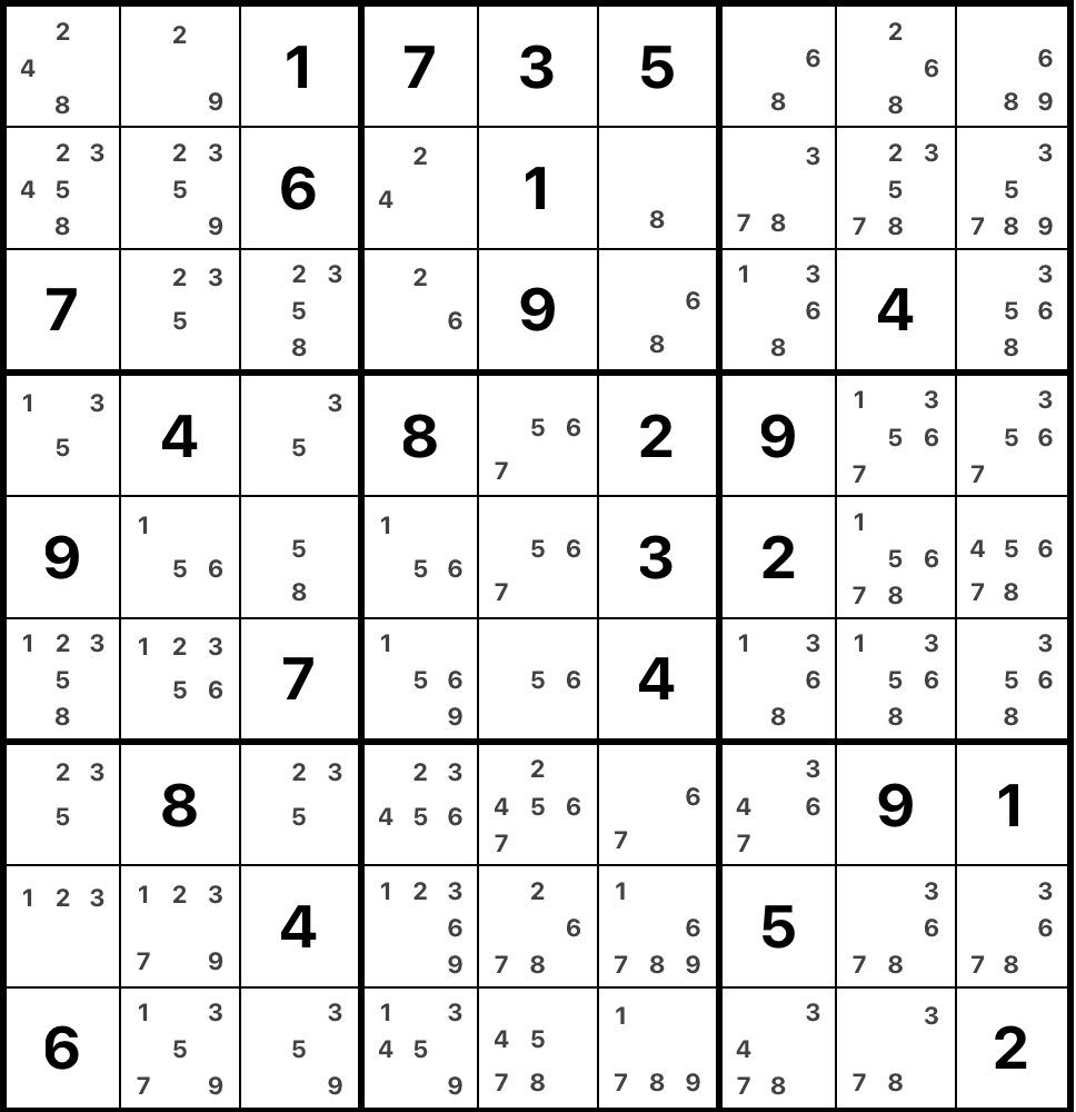
Here is an example of a sudoku and its solution.
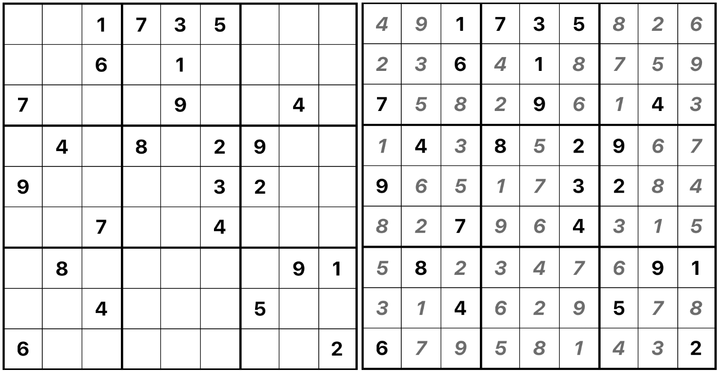
The grid is pre-filled with some digits, these are called clues. If a puzzle has a unique solution it is called valid. Interestingly, the number of clues (or the number of holes, if you wish) does not really measure the difficulty of a puzzle: while an almost filled grid will likely to be, but not necessarily, quite easy to finish, there are very sparse puzzles that are equally easy. For humans, the difficulty is usually measured by the techniques that are necessary to solve a given puzzle, and for the machines one tracks the depth of the search stack. This brings us to how one solves a sudoku.
How machines solve sudoku
The most straightforward and algorithmic way to solve a sudoku is to use backtracking. Put a digit in a cell, check that the placement doesn't contradict the rules: if not, then go to the next cell and do the same, if yes, then try another digit. If you tried all digits in this cell and all led to a contradiction, go to the previous cell and try another digit there. The process is recursive and naturally uses a stack.
We can reduce the search space considerably though by using some shortcuts. Let's look at a cell in row 2, column 6 in the example puzzle. How does one know what digit to put in there? In this case, we cannot put 6 and 1 to this cell because they are already present in the row. In the same way, we cannot place 5, 2, 3 and 4 because they are already in the column; the same works for 7, 3, 5, 1 and 9 because they are in the box of the cell. In the end, the only option left is 8. This is what is called a "naked single": a unique candidate in a cell. It is a hard constraint: when such a situation appears on the board there is no need to try other candidates in this cell as it will immediately lead to a contradiction. This is the simplest technique used by humans to solve a sudoku puzzle, and the simplest puzzles can be solved using this technique only.
In general, we define the set of candidates in a cell as the digits that are not present in cell's row, column and box. Having the set of candidates per cell helps a lot while solving a puzzle: in a way, in order to solve a sudoku one wants to reduce the candidate sets in every cell to a unique candidate. Here's the example grid with all candidates written down.

A different situation appears in row 3, column 7. In this cell, the candidates are 1, 3, 6, 8. Let's look at the candidates of other cells in the same row. We can notice that 1 is not a candidate in any of them (because it is present either in a row or a box). Thus, looking at this row, we can put 1 only in this cell. It's called "hidden single". It is a hard constraint as well and uniquely defines what digit to put. Usually, the "easy" puzzles can be solved using only these two techniques.
When these easy deductive placements are exhausted, the solver must fall back on search. It makes a guess, typically by selecting a cell with the fewest remaining candidates to minimize branching, and proceeds. If this branch leads to a contradiction, the algorithm pops the state from its search stack and tries the next candidate. A single guess usually unblocks a cascade of new forced placements. Therefore, the execution of this 'Norvig-style' solver produces a solving trace that looks like this: long sequences of deterministic, rule-based placements punctuated by occasional branching guesses and backtracking.
About additional solving techniques
It's also worth mentioning that humans usually don't use backtracking, at least not explicitly. Instead, more complex techniques are used, that are essentially guided tree search heuristics that allow to eliminate candidates from cells. One such example is "naked pair".

Look at the box 8 in the example. There are two cells with only 1 and 9 as candidates, call them A and B. Suppose that we put 1 to some other cell in this box. Then we have to put 9 in cell A, as it is the only candidate there. But now there are no candidates in cell B. Thus, 1 is not a candidate in any other cell in the box, and neither is 9. In general, if there is a pair of cells in a substructure that has the same two candidates, then these candidates cannot be candidates in other cells of this substructure. Basically, it is a "compressed" backtracking: instead of manually eliminating every candidate by backtracking, we apply a simple heuristic.
Setup: model and training
Following Giannoulis et al. and Shah et al., I train a causal transformer on reasoning traces. In order to describe these traces, we need first to describe the vocabulary.
Model vocabulary and traces
The model's vocabulary consists of two main categories:
- Placement tokens: there are 729 unique "cell-digit" tokens representing every possible placement (e.g.,
[R3C5=9]stands for placing a 9 in Row 3, Column 5). - Special tokens:
[clues_end]: marks the end of the initial puzzle description.[push]: indicates the solver is out of easy deductive moves and is making a "guess" to explore a branch in the search tree.[pop]: follows a guess that led to a contradiction, signaling the solver is discarding that branch and backing up the stack.[success]: appears when the board is valid and fully solved.[pad]: the standard padding token.
Using this vocabulary, we can now write down the solving process of the solver. Here is an example of what a trace looks like: [R1C1=5] ... [R2C4=3] [clues_end] [R3C5=9] [R6C8=4] [push] [R8C8=1] [pop] [push] [R8C8=2] ... [success]
Dataset and training
The puzzles for the training were taken from the sudoku-3m kaggle dataset. The traces were generated from these puzzles using a Norvig-style solver described in the previous section. An important modification to the standard solver is that a few randomizations are used, where usually the order is deterministic. Concretely, the order of "easy" constrained placements was randomized instead of following the row-major order. When there are several cells with the same number of candidates available for backtracking, the next one is chosen randomly. At last, the order of checking the candidates for backtracking is random as well.
I trained a causal transformer to predict the next token autoregressively in the solution trace. The traces were trimmed to 250 tokens, effectively not giving full traces for the hardest puzzles (which are only 0.9% of all traces). I used 2.7M puzzles for training, 150K for validation via random sampling and 150k for final test performance and subsequent use in probing experiments.
I tweaked the transformer architecture: I didn't use dropout and used pre-norm, as these choices are standard for modern models. For the rest I followed the choices of Giannoulis et al. and Shah et al.: 8 layers, 8 heads per transformer block, 576 model dimension and 3456 MLP dimension. After 6 epochs on the dataset (~2.5B tokens), the cell accuracy is 98.4% and the grid accuracy is 97.5% on the in-distribution puzzles. I trained the model on Google Colab TPU v6e, whole training took around 2 hours.
The code is available on github.
How is the state represented in the residual stream?
The main questions I wanted to answer:
- Does the model build a representation of different aspects of current state of the grid similarly to OthelloGPT?
- If yes, is the representation linear? Is the representation actually used?
Linear probes
A logistic regression probe is a pair of a vector
To map these representations, I trained probes after every transformer layer. I randomly chose 6,400 puzzles from the testing pool, training on 5,120 examples and evaluating on 1,280. For now, I probed activations exclusively at the [clues_end] token, as it serves as a common anchor point in all traces and doesn't yet involve the model making a decision.
Filled state
First, let's do a sanity check: does the model represent filled and empty cells in the residual stream? For every layer, I train 81 logistic regression probes, each answering the question "is the cell i currently filled"? After training the probes, I check the AUC and MSE per probe and then use the average scores per layer as the overall quality measure. As we can see in the figure, the probes get AUC 1.0 and MSE (aka Brier score) of 0.0 for all cells across in the mid-layers (3-6). Also there is a hint that the model has some representation of boxes, a structure that is only implicitly present.
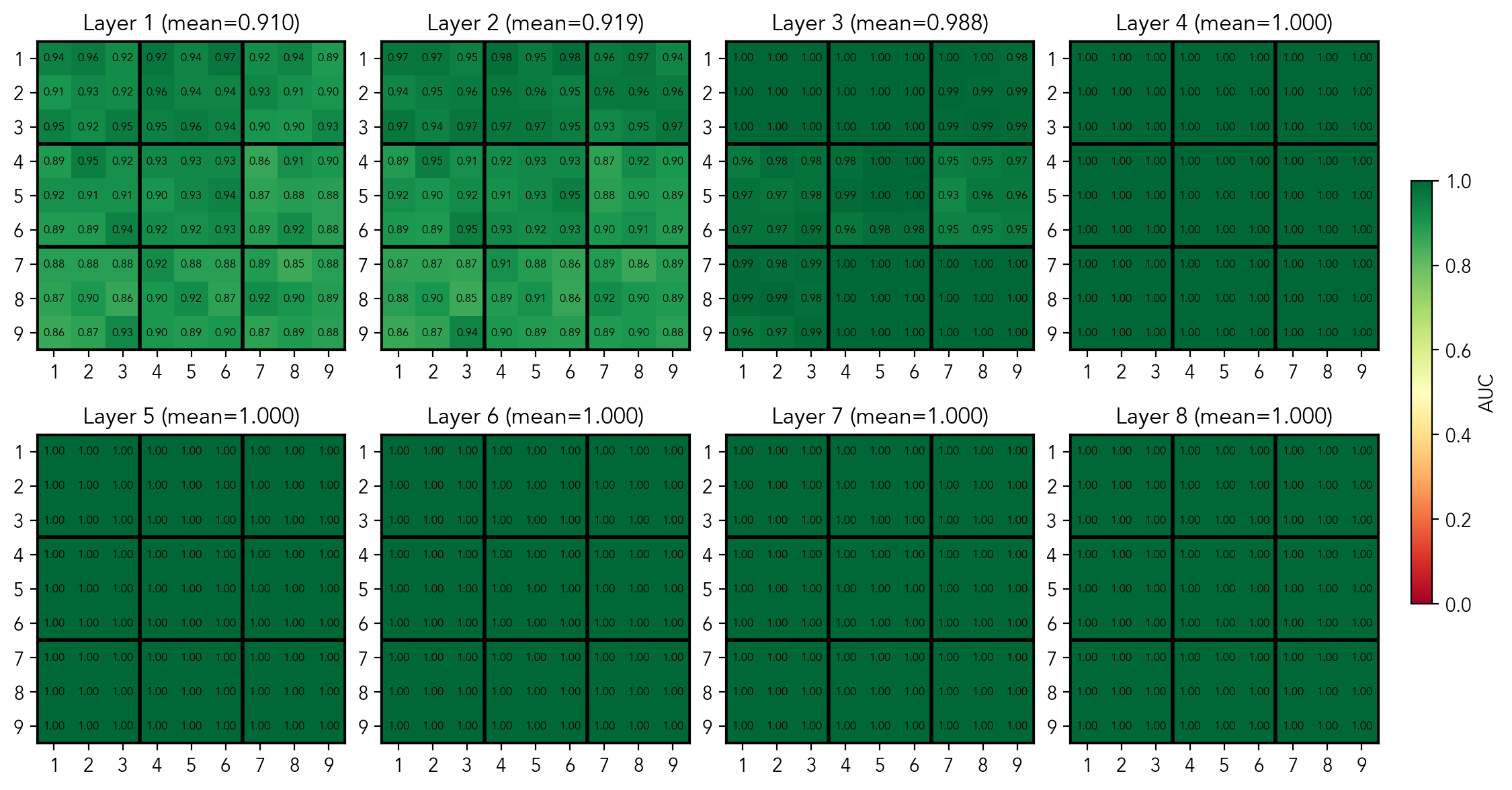
Per-cell AUC scores of the probes predicting if the cell is filled
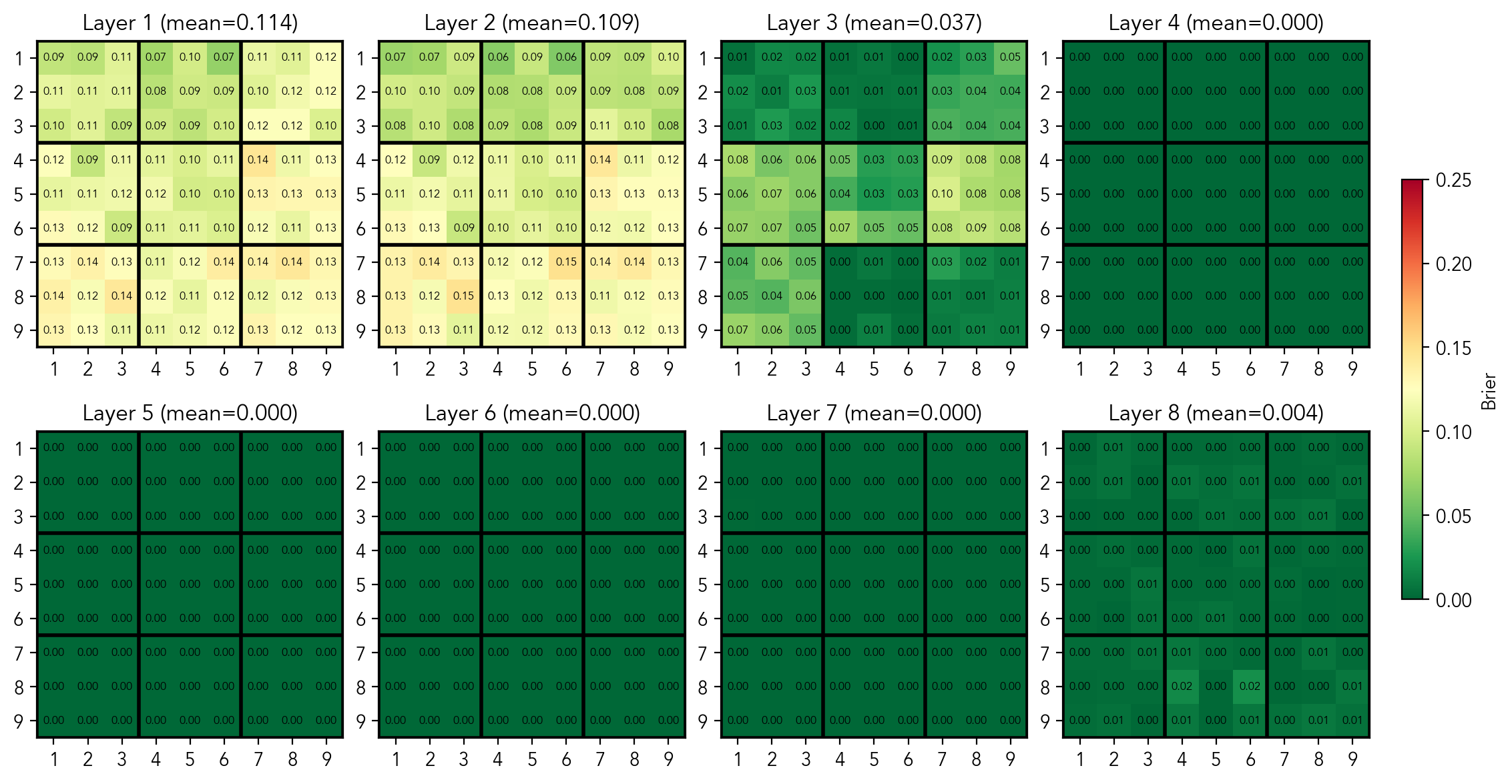
Per-cell MSE scores of the probes predicting if the cell is filled
State by cell
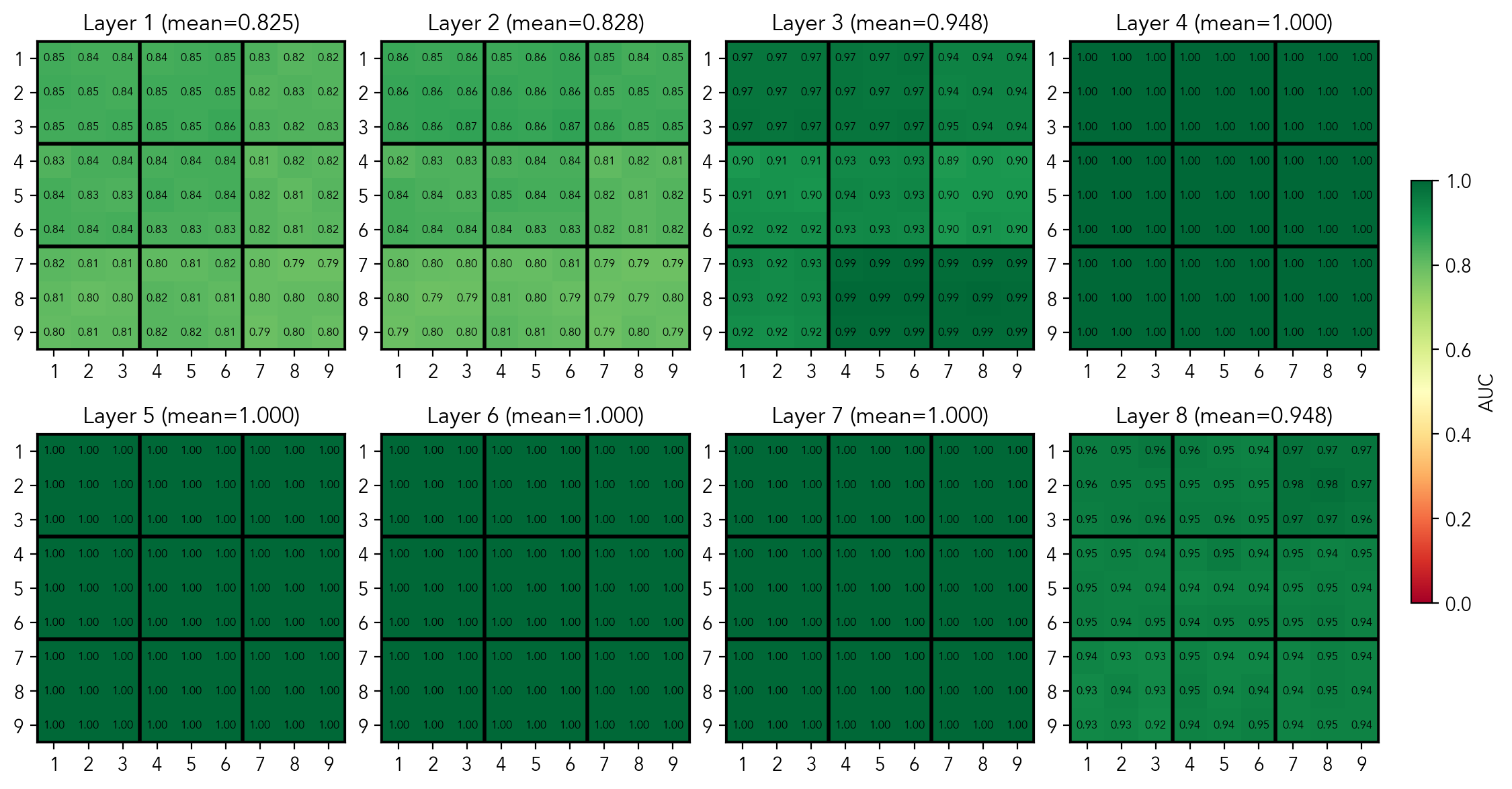
Next, does the model keep track of the digits in the cell? That is, does the model represent which digit is in a given cell, if there is one? To check this, I train probes that give the probability of "if the cell
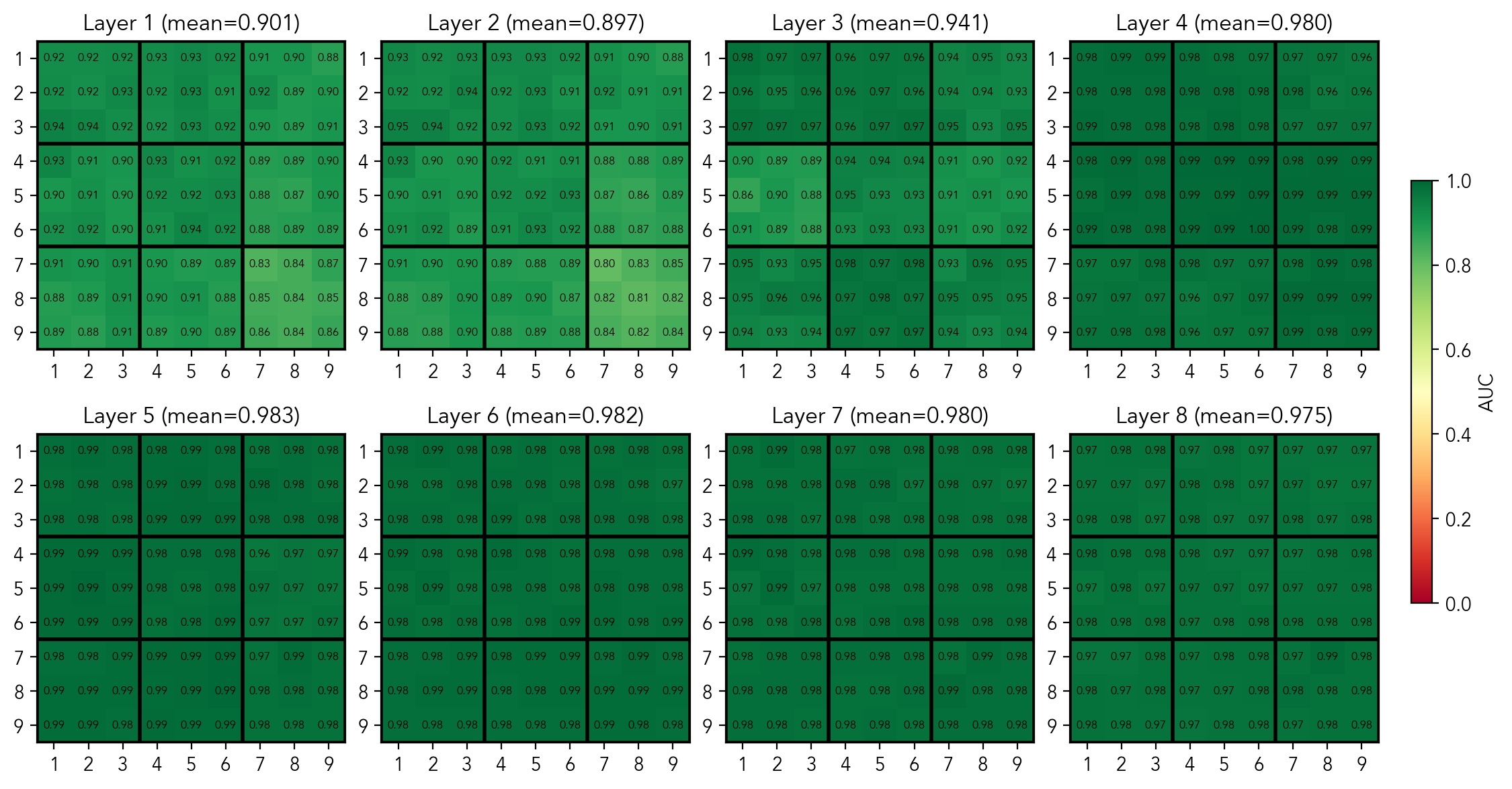
Mean per-cell AUC score of probes predicting the digit in a non-empty cell
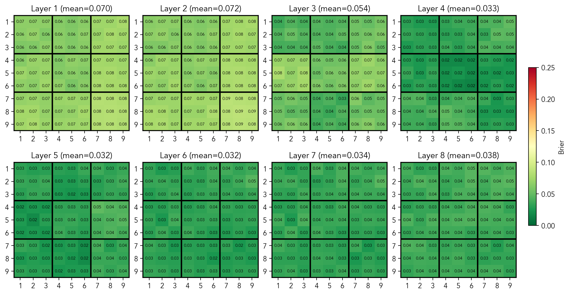
Mean per-cell MSE score of probes predicting the digit in a non-empty cell
Well, this is mildly confusing. The average AUC per cell of 0.983 is fairly high, but not perfect. It means that this data is not quite separable in the latent space. Moreover, the average MSE per cell of 0.032 at best is quite elevated. Remember that the clues describing the current state of the board are literally there right before the [clues_end] token. Let's leave it here for now, in a few moments we'll see that the does represent the board state, but using different building blocks.
Candidates per cell
While representing the current state of the board may be useful for solving the puzzle, keeping track of the candidates per cell is a big help for human solvers. Thus, the next question is: does the model represent candidates in a cell? Similarly to the state probes, I trained 729 probes that predict "if the cell i is empty, is digit d a valid candidate in this cell?".
Mean per-cell AUC score of probes predicting if the digit is a candidate in an empty cell
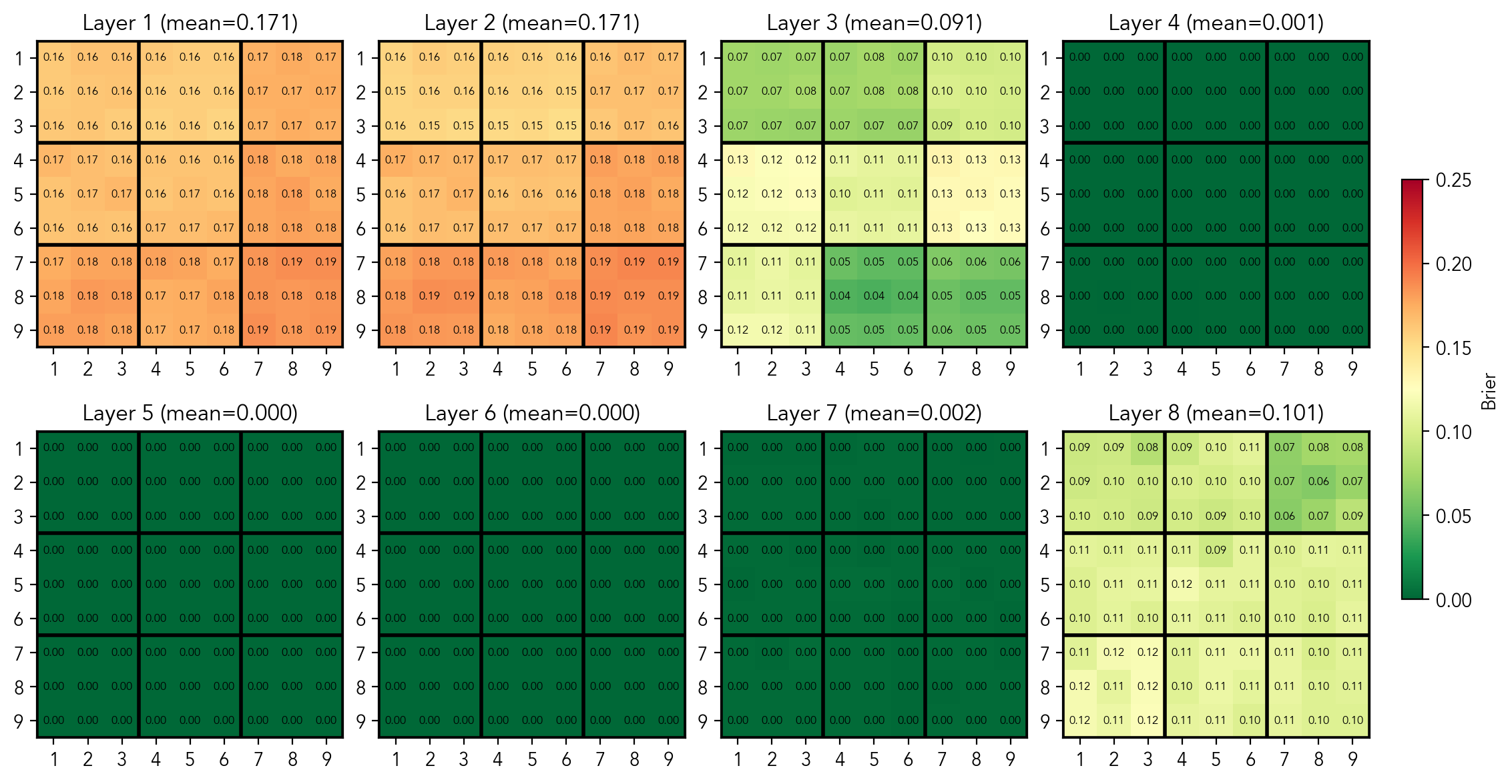
Mean per-cell MSE score of probes predicting if the digit is a candidate in an empty cell
As we can see, the model has a perfect linearly separable representation of this concept in the residual stream at the [clues_end] token in the middle layers. At this point I have trained 729 probes that predict if a digit is a candidate in a given cell. The prediction of a probe is given by
Before going to activation patching to see if the model actually uses this representation when predicting the next step, we'll take a look on the latent space. Concretely, we can look at the weight vectors of the probes to understand whether they encode independent features or share structure. For that, I plot a heat map of cosine similarity between a fixed
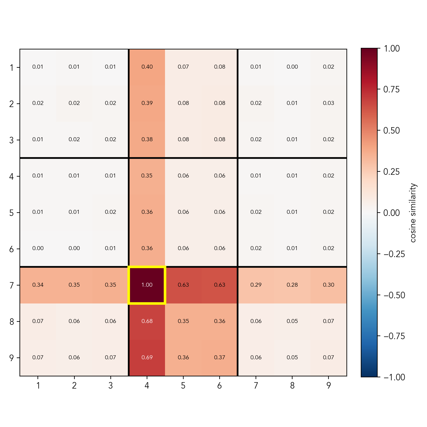
Cosine similarities between the candidate probe for cell (row 7, column 4), digit 2, and other candidate probes for digit 2
In the plot above you can see the similarity scores for the probe of cell (row 7, column 4), digit 2 (the same holds for other cells and digits). Clearly, the directions are not random. In fact, they are highly structured: the vector responsible for telling if digit 2 is a valid candidate in cell (row 7, column 4) is very much not orthogonal to the vectors telling if 2 is a valid candidate in: row 7, column 4, box 8; but is orthogonal to the vectors of other unrelated cells. Moreover, there is an additive structure: the cells that simultaneously belong to the box and the row/column (e.g. row 8, column 3, score = 0.68) get approximately the sum of the scores of cells that are either in the box, but not in row/column (e.g row 9, column 5, score=0.36), and cells that are not in the box, but in the row/column (e.g row 7, column 7, score=0.29). There is also a slight non-orthogonality with the cells that share "mini-rows" or "mini-columns", i.e. the rows or columns that go through the box the cell belongs to.
This is, in fact, a strong indication that candidates are encoded by substructure, rather than by individual cell. It's quite fascinating: I brought my own bias into the analysis by assuming the cell was the fundamental building block, but the model clearly learned a different geometry. Could it be that the transformer represents the board state as a combination of substructures, bypassing individual cells? That would elegantly explain why our per-cell state probes weren't linearly separable. Let's test this hypothesis.
State per substructure
There are 27 substructures in total (9 rows/column/boxes). For each, we train 9 probes that predict if digit is present in the substructure. The candidates probe for a substructure is equivalent to the state probe: if a digit is not present, then it is a candidate, by definition. The probes achieve the perfect AUC of 1.0 and MSE of 0.0 for all 27 substructures, without misclassification. In the plots, the scores per substructure for the layer 4 are given.
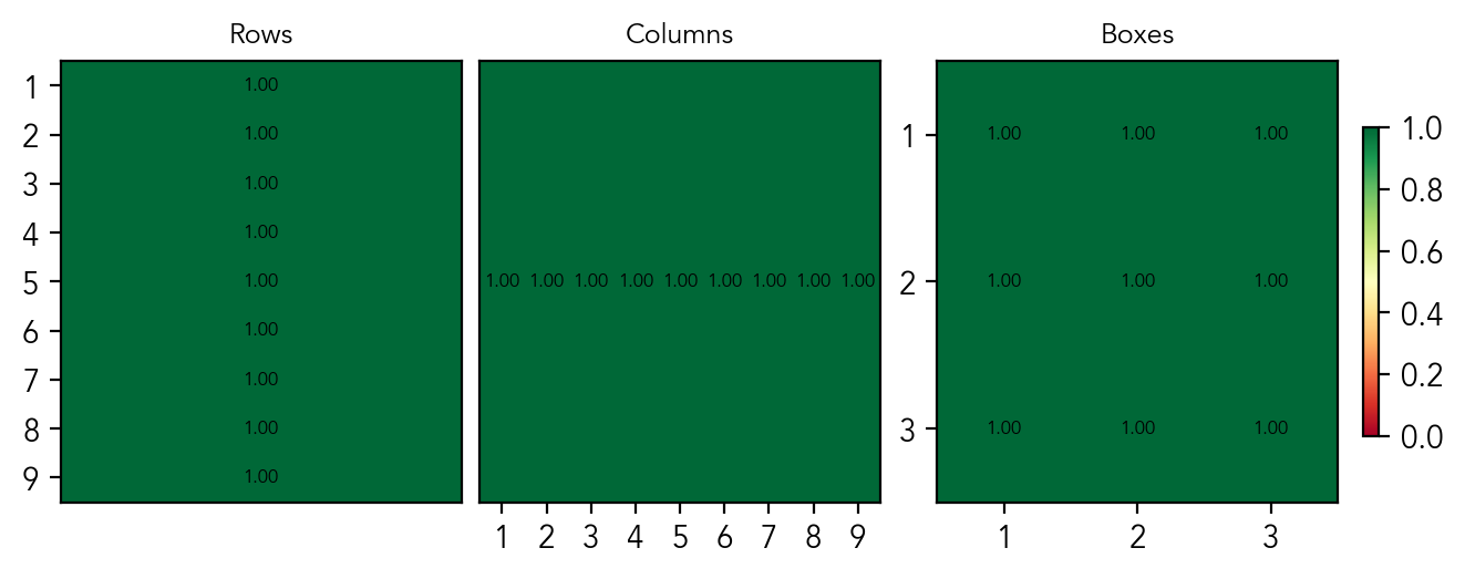
Mean per-substructure AUC score of probes predicting if a digit is present in a substructure
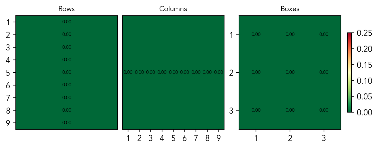
Mean per-substructure MSE score of probes predicting if a digit is present in a substructure
This is the main result: these scores prove that the board state exists as a linear representation in the residual stream. Surprisingly, the model completely abstracts away the notion of individual cells, instead learning to "see" the grid's sub-structures. It explains the non-perfect scores of the probes at the cell level: the data is simply not linearly separable in the residual stream. The model extracts this sub-structure geometry purely from sequential traces (a challenge harder than Othello), which shows that a world model is actively built, and that it is optimized for constraint-solving rather than pure memorization. This means that transformers may recover task-relevant abstraction and don't simply gather statistics.
Does the model use the same latent space throughout the execution?
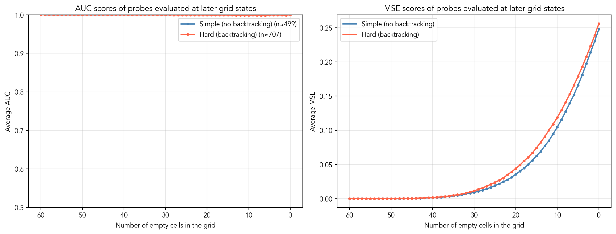
So far, I have only looked at probes trained and tested on the [clues_end] token. Naturally, we want to know if we can use these same probes to examine the latent representation later in the solution trace, especially to analyze the backtracking mechanism.
When we evaluate these initial probes on later tokens, we see that the average AUC score remains a perfect 1.0 throughout the entire solving process, proving that the latent space and the learned directions remain completely consistent. However, the MSE steadily increases as the grid fills up. The main reason for this drop in calibration is the bias term in the logistic regression: as candidates are eliminated, their base rate of appearing changes (in the beginning, a digit is a candidate in 40% of the cases, after 30 steps it is only in 10%). Thus, the probes simply need recalibration when used at later steps.
Activation patching
Now, we will answer the second question: does the model actually use the representation to decide what token to put next? I'll show what happens to the output probabilities when we suppress a direction associated to a (substructure, digit) pair in the residual stream. I'll also use that as an opportunity to look at some aspects of how these probabilities relate to the techniques used to solve a puzzle. Throughout, I apply the patching at layer 4, but the results hold at any layer. Concretely, for a given substructure
When we look at the probabilities that the model outputs, it exists in two modes: either the probability concentrated near 1.0 at one token, or it is (unevenly) distributed over several tokens. Let's start with the former.
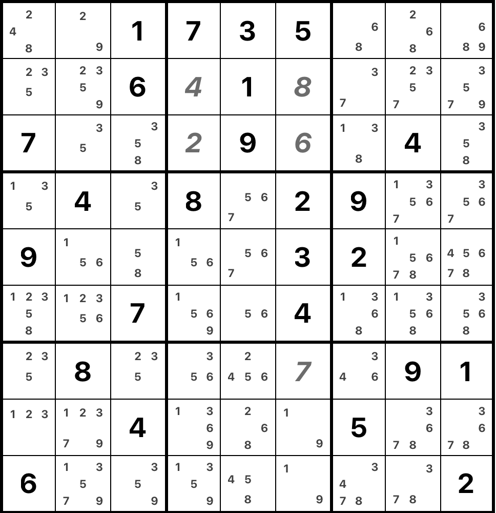
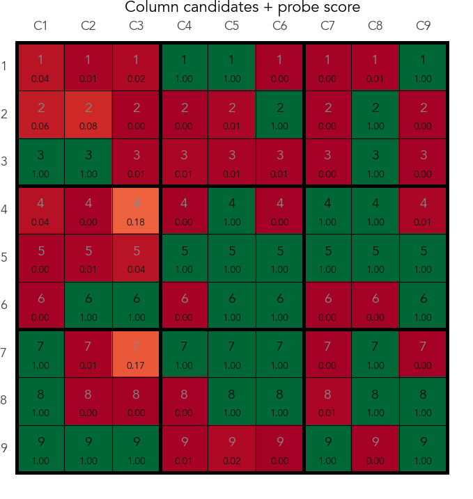
This is the puzzle from the introduction. It has only one "naked single" cell: row 2, column 6 contains a unique candidate 8. The model wants to fill this cell with 8, with the probability almost 1. If you look at other top candidates, though the probabilities are negligible, you can see that many of them point at the same cell.
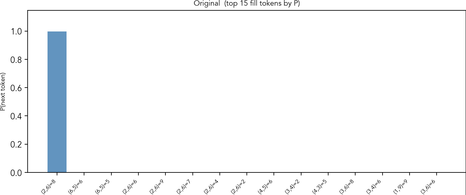
Output probabilities given by the model before patching
When we subtract the probe vector of the row 2, digit 8, these are the changed probabilities:
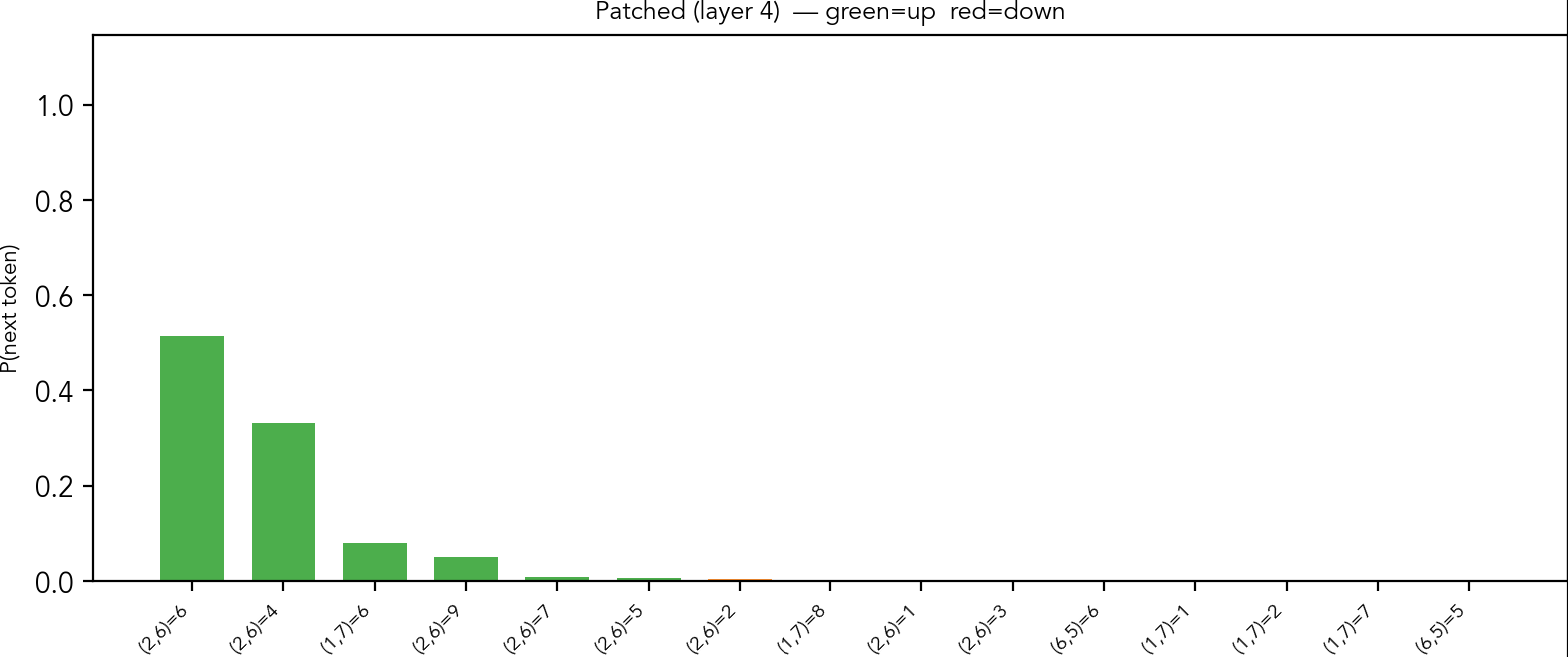
Output probabilities given by the model after subtracting (row 2, digit 8) token from activations after layer 4
The model now assigns a tiny probability to the original, instead giving more weight to other digits at the same cell. I hypothesize that it means there are two circuits in action: one suggests where to place the next token, and other suggests what to place. As "naked single" is quite easy to see once one has candidates representation, it may be difficult to suppress the "where" part of the circuit.
We observe the same for patching of the digit in the column and the box.
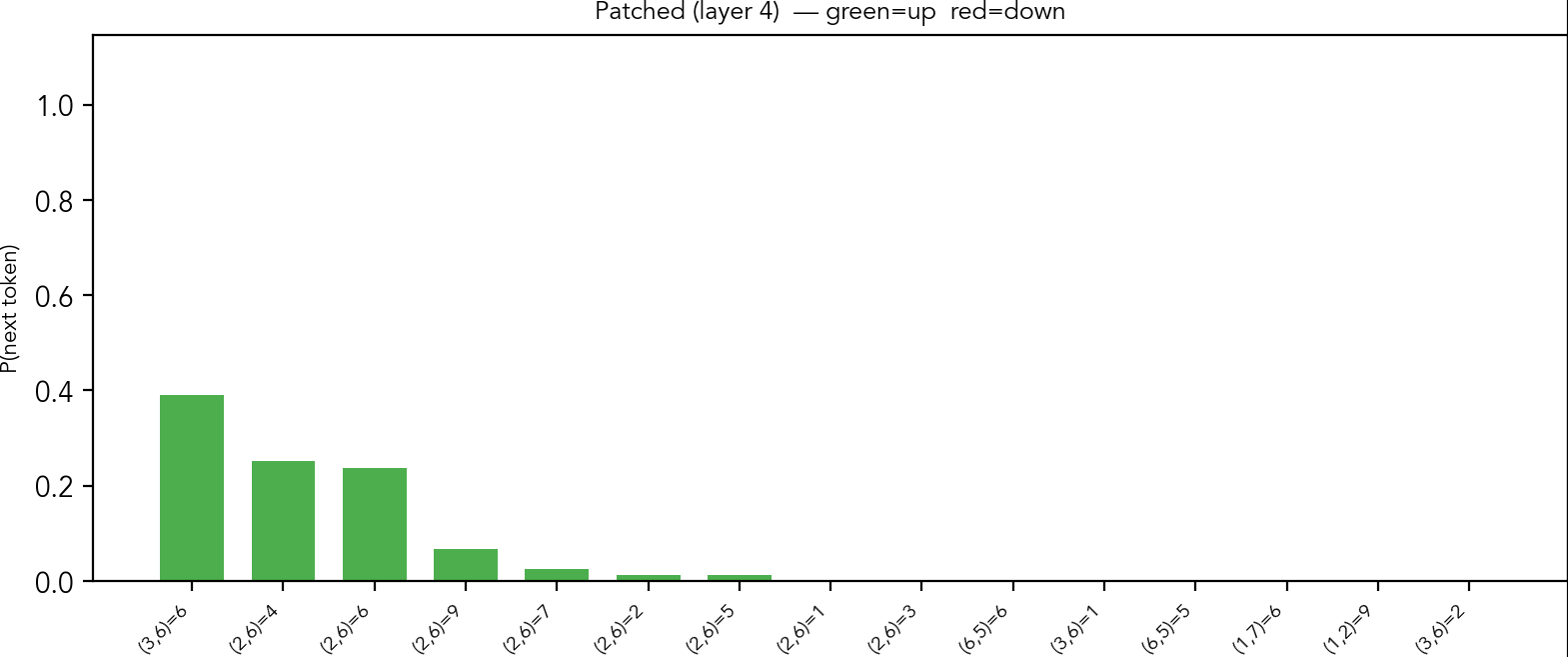
Output probabilities given by the model after patching using (column 6, digit 8) probe vector
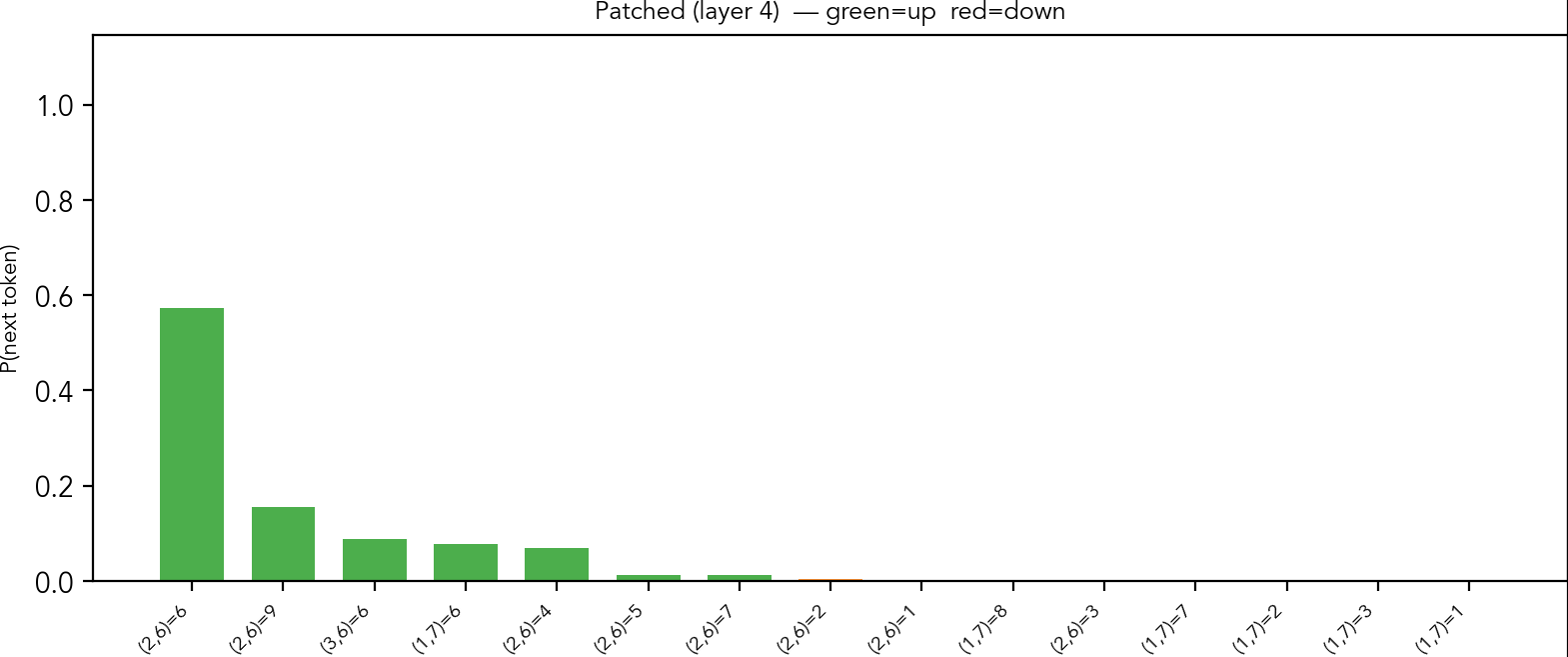
Output probabilities given by the model after patching using (box2, digit 8) probe vector
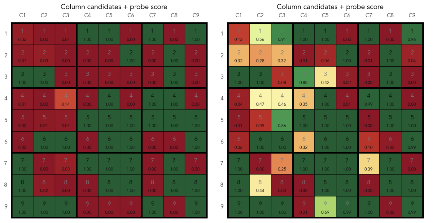
Following the correct placements, in the next steps the model consistently prefers to put digits indicated by the "single naked" strategy. After five steps, we arrive at the following state of the board.
Here, the next easy constrained placements are the "hidden singles". As we can see,
the model now spreads the probability mass across several tokens.
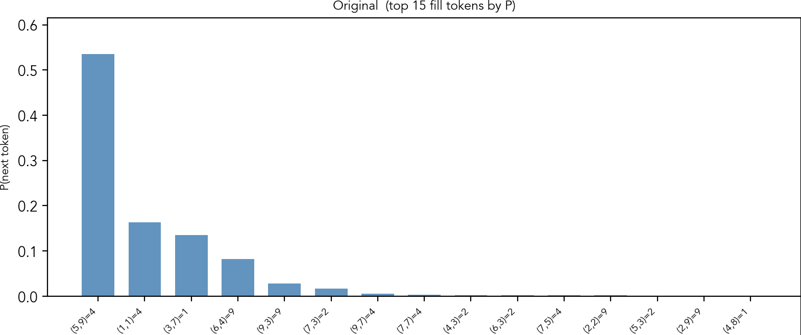
We can assess the guesses: four at (row 5, col 9) is a hidden single in its row, column and box at the same time. Four at (1,1) is a hidden single in its row, column and box as well. One at (3,7) is a hidden single in row and box; nine at (6,4) is a hidden single in the row and the box. Nine at (9,3) is a hidden single in its column only; two at (7,3) is hidden single in its column only. Four at (9,7) is a correct placement, but cannot be explained by a simple strategy. There are some other hidden singles that are not in the top predictions.
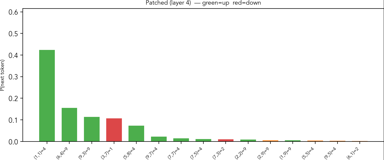
When the column 9, digit 4 patching is applied, it pushes other correct guesses up, but also confuses the model, as we see in the figure. Now, it suggests placing 4 at position (5,8), that is, the same row as in the correct prediction, but a different column.
All this indicates that the model actively uses representations to produce the final tokens.
Unembedding matrix
As the last evidence of the model building a robust internal representation of the grid and learning the rules of sudoku, I'll plot the pairwise cosine similarity of the vectors of the unembedding matrix.
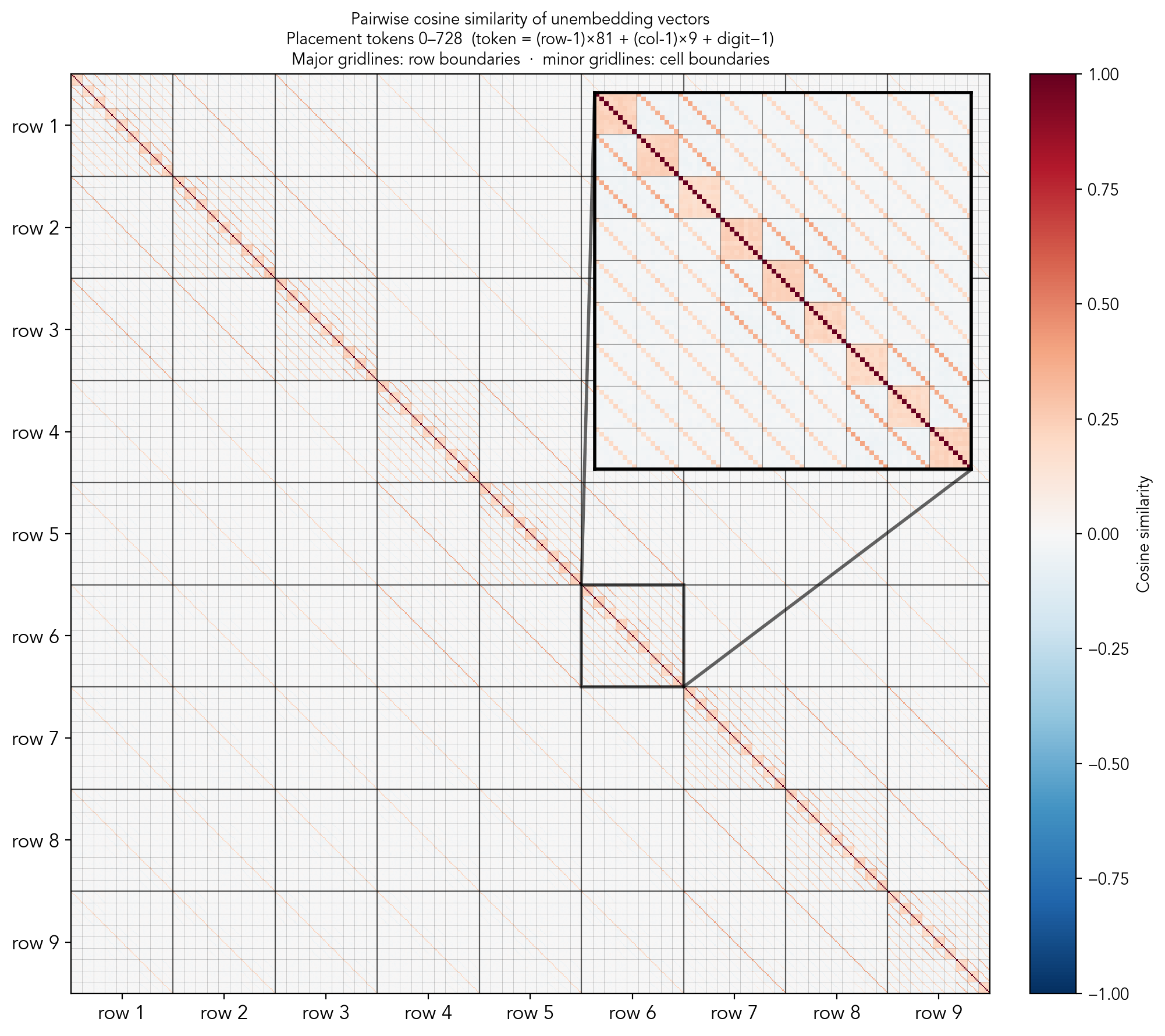
Here we look at the cosine similarity of 729 unembedding vectors. Each of the nine big cells is a row, each small square is a column, and the smallest squares are digits.
A zoomed part in picture for the intersection of row 6 and row 6, that is the similarities of all vectors that place a digit in the row 6. Tokens here all share the row, but may be of different columns or different digits. Looking at the scores, the tokens group into several clusters defined by whether they share row, column, box and digit. (If two tokens share the row and the column, it means they correspond to the same cell, so they must share the box). Overall, we can see that the scores are very structured and definitely not random. Moreover, there is a stratification, the pairs from the groups I described get almost identical similarity scores, as we can see in the next table.
Row | Col | Box | Digit | mean sim | n pairs |
|---|---|---|---|---|---|
diff | diff | diff | diff | -0.0003 ± 0.0074 | 349,920 |
same | diff | diff | diff | -0.0181 ± 0.0072 | 34,992 |
diff | same | diff | diff | -0.0176 ± 0.0074 | 34,992 |
diff | diff | same | diff | -0.0060 ± 0.0073 | 23,328 |
same | diff | same | diff | -0.0317 ± 0.0079 | 11,664 |
diff | same | same | diff | -0.0350 ± 0.0083 | 11,664 |
same | same | same | diff | 0.2158 ± 0.0223 | 5,832 |
diff | diff | diff | same | -0.0206 ± 0.0203 | 43,740 |
same | diff | diff | same | 0.2004 ± 0.0210 | 4,374 |
diff | same | diff | same | 0.1962 ± 0.0234 | 4,374 |
diff | diff | same | same | 0.0712 ± 0.0226 | 2,916 |
same | diff | same | same | 0.3645 ± 0.0251 | 1,458 |
diff | same | same | same | 0.3788 ± 0.0259 | 1,458 |
same | same | same | same | 1.0 | 729 |
If we swap the rows and columns, the scores are almost the same, which may indicate that the model allocates equal importance to rows and columns. We can also see that the vectors for the same cell but different digits have a common component: this may explain why, when suppressing the direction for a unique guess, the model instead outputs other digits for the same cell.
Backtracking
The following is a preliminary result. So far I mainly focused on simple puzzles that don't use backtracking. However, while looking at the traces that do use backtracking, I noticed that the model actively suppresses the representation of candidates after a failed branch of exploration.
Take the probes that are trained to predict the candidates per substructure. The model starts backtracking by writing the [push] token and then a token for digit d at cell i. Eventually, it reaches a contradiction and pops the stack by writing [pop]. What I observe is that at the next [push], a probe for a substructure that contains i indicates that d is no longer a candidate in this substructure, even though the state of the board is effectively rolled back by the model. After placing the next guess, d is again predicted to be a valid candidate in that substructure.
Here's an example. In a puzzle, after exhausting all easy constrained placements, the model has to guess. The real valid candidates in cell (row 6, column 7) are 1 and 5, and it's the cell that contains the lowest number of candidates, so the model chooses there. The model emits [push] token and a probe predicts that 5 is a candidate in column 7. The model then puts 5 to cell (6,7). After several steps it fails, outputs the [pop] token and the next [push] token. The probe at the second [push] shows that 5 is no longer a candidate in column 7. Right after placing the next guess, that is 1 at cell (6,7), the probe shows that 5 is again a candidate in column 7.
Predictions for (column, digit) pairs at the first and second [push] tokens
Probe predictions after the second [push] token
(vertical axis - column, horizontal axis - digit)
Conclusion
In this post I wanted to find whether a transformer trained on sudoku solving traces builds an internal world model, following the line of research started by OthelloGPT. The answer is yes, but the model's representation is organized in a way different both from OthelloGPT and my first naive assumption. Where OthelloGPT maintains a per-cell representation, the sudoku transformer abstracts away individual cells, and instead represents the board state per substructure: whether each digit is present in each row, column, and box. This representation mirrors the structure of the puzzle constraints, suggesting that the model has recovered a task-relevant abstraction.
These results provide further evidence for the linear representation hypothesis: the board state is encoded as linear directions in the residual stream, recoverable by simple logistic regression probes. But they also refine it in an interesting way. The features that are linearly separable are not the ones most intuitive to a human observer (which digit is in which cell), but the ones most useful for constraint propagation (which digits are present in which substructure).
This carries a methodological lesson as well. Per-cell state probes achieved good, but imperfect scores, which I initially interpreted as an incomplete representation. In fact, the representation was there, it was simply organized around a different unit of analysis than the one I assumed. I believe this is worth keeping in mind for future interpretability work: a probe's failure may say more about the experimenter's ontology than the model's.
Activation patching confirmed that the substructure representation is actually used for prediction: suppressing a single (substructure, digit) direction causally changes the model's output probabilities. The patching also showed a preliminary insight: the model appears to separate "where to place" from "what to place," because suppressing the digit direction for a substructure shifts probability mass to other digits at the same cell rather than to other cells entirely.
There are some important limitations. All probing results in this post are based on activations at the [clues_end] token, a convenient but early anchor point. The backtracking analysis is rudimentary: I showed an example where the model suppresses candidates for a failed guess between [pop] and the next [push], but the mechanism behind this suppression is unexplored.
Part 2 will cover the training process, dataset construction, and model performance in more detail. Part 3 will dig into the mechanics: how do attention patterns implement candidate tracking? What circuits mediate the "where" and "what" separation? And most concretely, how does the model implement backtracking?
LLM disclosure
Claude was used to write the code for the experiments, and Gemini was used to correct the grammar in the post.
Discuss