How Snowflake ML, XGBoost, the Model Registry, and ML Observability let you go from raw transactions to a monitored fraud scorer without ever leaving your data platform
Fraud doesn’t wait. A transaction hits in milliseconds, and your window to flag it before the funds move is even shorter. Yet most fraud-detection stacks still look like an archaeology dig — raw data in a warehouse, feature engineering on someone’s laptop, a pickled model emailed to a DevOps team, and a monitoring dashboard bolted on as an afterthought.

This article walks through a complete, production-grade alternative: a seven-stage ML pipeline built entirely inside Snowflake. Every line of code below runs in a Snowflake Notebook. Your model lives next to your data. Your predictions land in a governed table. Your drift checks run on a daily schedule. No context switching. No data copies leaving the platform.
Why Build ML Inside Snowflake?
The core problem with external ML stacks is data gravity. Your transaction data lives in Snowflake — governed, secured, optimised. The moment you pull it into a local environment or ship it to an external training cluster, you’ve broken the chain: data leaves your security perimeter, lineage gaps appear, and the operational distance between “where data lives” and “where the model runs” becomes a recurring liability.
Snowflake ML eliminates that gap. Your Snowpark session is your compute layer. Experiment tracking, model registry, batch inference, and observability all share the same platform and the same access controls you’ve already defined.
The Pipeline at a Glance
Seven stages, one platform:
- Data loading & EDA — Understand the class imbalance and feature distributions
- Feature engineering — Create risk signals the model can actually learn from
- Model training — XGBoost with class-weight handling and experiment tracking
- Evaluation — ROC-AUC, Average Precision, confusion matrix, threshold optimisation
- Model Registry — Register a versioned model with attached metrics
- Batch inference — Score new transactions using the registered model
- ML Observability — Set up a model monitor for drift and score distribution
Step 1: Session Setup
import warnings
warnings.filterwarnings('ignore')
import numpy as np
import pandas as pd
import matplotlib.pyplot as plt
from snowflake.snowpark.context import get_active_session
session = get_active_session()
session.sql("USE DATABASE ML").collect()
session.sql("USE SCHEMA PRODUCTION").collect()
print(f"Session ready: {session.get_current_database()}.{session.get_current_schema()}")
get_active_session() binds you to the Snowflake Notebook's existing session — no credentials to manage, no connection strings to rotate.
Step 2: Data Loading & EDA
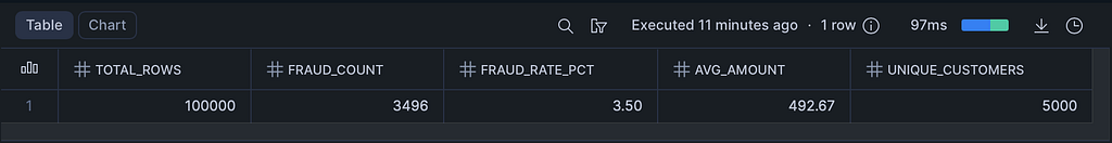
Start with a SQL summary to get the fraud rate and dataset shape before pulling anything into memory:
%%sql -r data_summary
SELECT COUNT(*) AS TOTAL_ROWS,
       SUM(IS_FRAUD) AS FRAUD_COUNT,
       ROUND(SUM(IS_FRAUD) / COUNT(*) * 100, 2) AS FRAUD_RATE_PCT,
       ROUND(AVG(TRANSACTION_AMOUNT), 2) AS AVG_AMOUNT,
       COUNT(DISTINCT CUSTOMER_ID) AS UNIQUE_CUSTOMERS
FROM ML.PRODUCTION.TRANSACTIONS
Peek at a few raw rows to understand the schema:
%%sql -r sample_data
SELECT * FROM ML.PRODUCTION.TRANSACTIONS LIMIT 5


Then pull the full dataset into Pandas for EDA:
df = session.table("ML.PRODUCTION.TRANSACTIONS").to_pandas()
print(f"Dataset shape: {df.shape}")
print(f"\nFraud distribution:")
print(df['IS_FRAUD'].value_counts())
print(f"\nFraud rate: {df['IS_FRAUD'].mean()*100:.2f}%")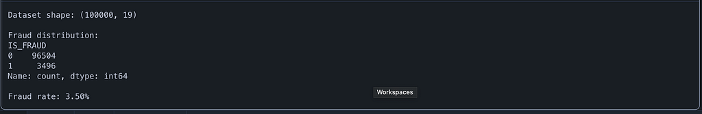
Expect fraud rates in the 0.5%–2% range on realistic transaction datasets. That class imbalance is the central modelling challenge — and we’ll address it directly in the XGBoost parameters.
Now visualise the key patterns across six dimensions:
fig, axes = plt.subplots(2, 3, figsize=(18, 10))
df['IS_FRAUD'].value_counts().plot(kind='bar', ax=axes[0, 0], color=['steelblue', 'salmon'])
axes[0, 0].set_title('Fraud vs Legitimate')
axes[0, 0].set_xticklabels(['Legitimate', 'Fraud'], rotation=0)
for label, color in [(0, 'steelblue'), (1, 'salmon')]:
    subset = df[df['IS_FRAUD'] == label]
    axes[0, 1].hist(subset['TRANSACTION_AMOUNT'], bins=50, alpha=0.6, label=f"{'Fraud' if label else 'Legit'}", color=color)
axes[0, 1].set_title('Transaction Amount Distribution')
axes[0, 1].legend()
axes[0, 1].set_xlim(0, 5000)
fraud_by_channel = df.groupby('CHANNEL')['IS_FRAUD'].mean().sort_values(ascending=False)
fraud_by_channel.plot(kind='bar', ax=axes[0, 2], color='coral')
axes[0, 2].set_title('Fraud Rate by Channel')
axes[0, 2].set_ylabel('Fraud Rate')
axes[0, 2].tick_params(axis='x', rotation=45)
fraud_by_hour = df.groupby('HOUR_OF_DAY')['IS_FRAUD'].mean()
axes[1, 0].plot(fraud_by_hour.index, fraud_by_hour.values, marker='o', color='coral')
axes[1, 0].set_title('Fraud Rate by Hour of Day')
axes[1, 0].set_xlabel('Hour')
axes[1, 0].set_ylabel('Fraud Rate')
fraud_by_category = df.groupby('MERCHANT_CATEGORY')['IS_FRAUD'].mean().sort_values(ascending=False)
fraud_by_category.plot(kind='bar', ax=axes[1, 1], color='coral')
axes[1, 1].set_title('Fraud Rate by Merchant Category')
axes[1, 1].tick_params(axis='x', rotation=45)
numeric_cols = ['TRANSACTION_AMOUNT', 'DEVICE_TRUST_SCORE', 'FAILED_TRANSACTIONS_LAST_24H',
                'VELOCITY_SCORE', 'DISTINCT_COUNTRIES_7D', 'CUSTOMER_CREDIT_SCORE']
corr_with_fraud = df[numeric_cols + ['IS_FRAUD']].corr()['IS_FRAUD'].drop('IS_FRAUD').sort_values()
corr_with_fraud.plot(kind='barh', ax=axes[1, 2], color='teal')
axes[1, 2].set_title('Correlation with Fraud')
plt.tight_layout()
plt.show()

These six panels reveal the patterns your features need to encode: the 00:00–05:00 risk window, channel-level fraud concentration, merchant category risk tiers, and which numeric columns correlate most strongly with IS_FRAUD.
Step 3: Feature Engineering
Raw transactional columns rarely have the signal density a fraud model needs. This block creates five composite features and one-hot encodes the categoricals:
df['AMOUNT_TO_AVG_RATIO'] = df['TRANSACTION_AMOUNT'] / (df['AVG_TRANSACTION_AMOUNT_30D'] + 1e-6)
df['IS_HIGH_RISK_HOUR'] = ((df['HOUR_OF_DAY'] >= 0) & (df['HOUR_OF_DAY'] <= 5)).astype(int)
df['RISK_COMPOSITE'] = (
    df['VELOCITY_SCORE'] * 0.3 +
    (1 - df['DEVICE_TRUST_SCORE']) * 0.3 +
    (df['FAILED_TRANSACTIONS_LAST_24H'] / 10) * 0.2 +
    (df['DISTINCT_COUNTRIES_7D'] / 5) * 0.2
)
df['LOG_AMOUNT'] = np.log1p(df['TRANSACTION_AMOUNT'])
df['CREDIT_SCORE_BIN'] = pd.cut(df['CUSTOMER_CREDIT_SCORE'], bins=[0, 500, 650, 750, 850], labels=[0, 1, 2, 3]).astype(int)
categorical_cols = ['CHANNEL', 'MERCHANT_CATEGORY', 'MERCHANT_COUNTRY', 'CARD_TYPE']
df_encoded = pd.get_dummies(df, columns=categorical_cols, drop_first=True, dtype=int)
print(f"Engineered dataset shape: {df_encoded.shape}")
print(f"New features: AMOUNT_TO_AVG_RATIO, IS_HIGH_RISK_HOUR, RISK_COMPOSITE, LOG_AMOUNT, CREDIT_SCORE_BIN")
Engineered dataset shape: (100000, 42)
New features: AMOUNT_TO_AVG_RATIO, IS_HIGH_RISK_HOUR, RISK_COMPOSITE, LOG_AMOUNT, CREDIT_SCORE_BIN
Why RISK_COMPOSITE? Individual risk signals — velocity, device trust, failed transactions, geographic spread — are correlated but incomplete in isolation. The composite collapses them into a single score while preserving their individual influence through the separate columns. Think of it as a hand-crafted prior probability signal that gives the model a head start.
Why LOG_AMOUNT? Transaction amounts are heavily right-skewed. Log-transforming compresses the tail, producing cleaner split points for the tree ensemble.
Then define the train/test split with stratification to preserve the fraud rate across both sets:
from sklearn.model_selection import train_test_split

drop_cols = ['TRANSACTION_ID', 'TRANSACTION_TIMESTAMP', 'IS_FRAUD']
feature_cols = [c for c in df_encoded.columns if c not in drop_cols]

X = df_encoded[feature_cols]
y = df_encoded['IS_FRAUD']

X_train, X_test, y_train, y_test = train_test_split(X, y, test_size=0.2, random_state=42, stratify=y)

print(f"Training set: {X_train.shape[0]} rows ({y_train.sum()} fraud)")
print(f"Test set:     {X_test.shape[0]} rows ({y_test.sum()} fraud)")
print(f"Features:     {X_train.shape[1]}")
Training set: 80000 rows (2797 fraud)
Test set:     20000 rows (699 fraud)
Features:     39
Step 4: Model Training with Experiment Tracking
Two things make this training block production-ready: scale_pos_weight handles class imbalance, and Snowflake's ExperimentTracking captures every run for reproducibility and comparison.
First, define the hyperparameter set:
from xgboost import XGBClassifier
from sklearn.metrics import (
    classification_report, confusion_matrix, roc_auc_score,
    precision_recall_curve, average_precision_score, f1_score
)

scale_pos_weight = (y_train == 0).sum() / (y_train == 1).sum()
params = {
    'n_estimators': 500,
    'max_depth': 6,
    'learning_rate': 0.05,
    'subsample': 0.8,
    'colsample_bytree': 0.8,
    'scale_pos_weight': scale_pos_weight,
    'min_child_weight': 5,
    'reg_alpha': 0.1,
    'reg_lambda': 1.0,
    'eval_metric': 'aucpr',
    'early_stopping_rounds': 50,
    'random_state': 42,
}
print(f"Class imbalance ratio (scale_pos_weight): {scale_pos_weight:.2f}")
print(f"Hyperparameters: {params}")
Class imbalance ratio (scale_pos_weight): 27.60
Hyperparameters: {'n_estimators': 500, 'max_depth': 6, 'learning_rate': 0.05, 'subsample': 0.8, 'colsample_bytree': 0.8, 'scale_pos_weight': 27.60207365033965, 'min_child_weight': 5, 'reg_alpha': 0.1, 'reg_lambda': 1.0, 'eval_metric': 'aucpr', 'early_stopping_rounds': 50, 'random_state': 42}
Why scale_pos_weight? If fraud is 1% of your data, an uncalibrated model learns to predict "not fraud" 99% of the time and achieves 99% accuracy while being completely useless. scale_pos_weight tells XGBoost to treat each fraud case as roughly N times more important, where N is the imbalance ratio.
Why aucpr over auc? On imbalanced datasets, ROC-AUC can be misleadingly optimistic — it incorporates the true-negative rate, which is inflated when legitimate transactions dominate. Average Precision (area under the precision-recall curve) is far more discriminating for rare-event detection.
Now train inside an experiment run:
from snowflake.ml.experiment import ExperimentTracking

exp = ExperimentTracking(session=session)
exp.set_experiment("fraud_detection_experiment")

with exp.start_run("xgboost_v1"):
    exp.log_params(params)
    model = XGBClassifier(**params)
    model.fit(
        X_train, y_train,
        eval_set=[(X_test, y_test)],
        verbose=50
    )

print(f"\nTraining complete. Best iteration: {model.best_iteration}")
[0] validation_0-aucpr:0.46674
[50] validation_0-aucpr:0.48302
[57] validation_0-aucpr:0.48405
Training complete. Best iteration: 7
🏃 View run XGBOOST_V1 at: https://app.snowflake.com/_deeplink/#/experiments/databases/ML/schemas/PRODUCTION/experiments/FRAUD_DETECTION_EXPERIMENT/runs/XGBOOST_V1
🧪 View experiment at: https://app.snowflake.com/_deeplink/#/experiments/databases/ML/schemas/PRODUCTION/experiments/FRAUD_DETECTION_EXPERIMENT
Every parameter, metric, and model artefact from this run is tracked inside Snowflake — no MLflow server to manage, no external experiment store.
Step 5: Evaluation
y_pred = model.predict(X_test)
y_proba = model.predict_proba(X_test)[:, 1]

roc_auc = roc_auc_score(y_test, y_proba)
avg_precision = average_precision_score(y_test, y_proba)
f1 = f1_score(y_test, y_pred)
metrics = {
    'roc_auc': float(roc_auc),
    'average_precision': float(avg_precision),
    'f1_score': float(f1),
    'best_iteration': int(model.best_iteration),
}
print("\n" + "="*50)
print("MODEL EVALUATION RESULTS")
print("="*50)
print(f"ROC AUC:           {roc_auc:.4f}")
print(f"Average Precision: {avg_precision:.4f}")
print(f"F1 Score:          {f1:.4f}")
print(f"\nClassification Report:")
print(classification_report(y_test, y_pred, target_names=['Legitimate', 'Fraud']))
==================================================
MODEL EVALUATION RESULTS
==================================================
ROC AUC:           0.7275
Average Precision: 0.4907
F1 Score:          0.5096

Classification Report:
              precision    recall  f1-score   support

  Legitimate       0.98      0.99      0.98     19301
       Fraud       0.58      0.45      0.51       699

    accuracy                           0.97     20000
   macro avg       0.78      0.72      0.75     20000
weighted avg       0.97      0.97      0.97     20000
Visualise the confusion matrix, feature importances, and the precision-recall curve together:
fig, axes = plt.subplots(1, 3, figsize=(20, 5))

cm = confusion_matrix(y_test, y_pred)
im = axes[0].imshow(cm, cmap='Blues')
for i in range(2):
    for j in range(2):
        axes[0].text(j, i, f'{cm[i, j]:,}', ha='center', va='center', fontsize=14, fontweight='bold')
axes[0].set_xticks([0, 1])
axes[0].set_yticks([0, 1])
axes[0].set_xticklabels(['Legitimate', 'Fraud'])
axes[0].set_yticklabels(['Legitimate', 'Fraud'])
axes[0].set_xlabel('Predicted')
axes[0].set_ylabel('Actual')
axes[0].set_title('Confusion Matrix')
plt.colorbar(im, ax=axes[0])
importances = model.feature_importances_
feature_importance_df = pd.DataFrame({'feature': feature_cols, 'importance': importances})
top_features = feature_importance_df.nlargest(15, 'importance')
top_features.plot(kind='barh', x='feature', y='importance', ax=axes[1], color='teal', legend=False)
axes[1].set_title('Top 15 Feature Importances')
axes[1].set_xlabel('Importance')
precision, recall, thresholds = precision_recall_curve(y_test, y_proba)
axes[2].plot(recall, precision, color='coral', linewidth=2)
axes[2].fill_between(recall, precision, alpha=0.2, color='coral')
axes[2].set_xlabel('Recall')
axes[2].set_ylabel('Precision')
axes[2].set_title(f'Precision-Recall Curve (AP={avg_precision:.3f})')
axes[2].set_xlim([0, 1])
axes[2].set_ylim([0, 1])
plt.tight_layout()
plt.show()

Threshold Optimisation
Don’t stop at the default 0.5 threshold. Sweep thresholds to find the operating point that maximises F1:
optimal_threshold = 0.5
best_f1 = 0
for threshold in np.arange(0.1, 0.9, 0.01):
    y_pred_t = (y_proba >= threshold).astype(int)
    f1_t = f1_score(y_test, y_pred_t)
    if f1_t > best_f1:
        best_f1 = f1_t
        optimal_threshold = threshold
y_pred_optimal = (y_proba >= optimal_threshold).astype(int)
print(f"Optimal threshold: {optimal_threshold:.2f}")
print(f"F1 at optimal threshold: {best_f1:.4f}")
print(f"\nClassification Report at optimal threshold:")
print(classification_report(y_test, y_pred_optimal, target_names=['Legitimate', 'Fraud']))
metrics['optimal_threshold'] = float(optimal_threshold)
metrics['f1_at_optimal'] = float(best_f1)
print(f"Updated metrics: {metrics}")
Optimal threshold: 0.58
F1 at optimal threshold: 0.5874

Classification Report at optimal threshold:
              precision    recall  f1-score   support

  Legitimate       0.98      1.00      0.99     19301
       Fraud       0.90      0.43      0.59       699

    accuracy                           0.98     20000
   macro avg       0.94      0.72      0.79     20000
weighted avg       0.98      0.98      0.98     20000

Updated metrics: {'roc_auc': 0.7274712577991356, 'average_precision': 0.49069855019666647, 'f1_score': 0.5096463022508039, 'best_iteration': 7, 'optimal_threshold': 0.5799999999999997, 'f1_at_optimal': 0.58743961352657}
Practitioner note: In fraud, false positives and false negatives carry asymmetric business costs. A false positive blocks a legitimate transaction and angers a customer. A false negative lets fraud through and costs real money. The threshold sweep lets you find the exact operating point that matches your business’s cost ratio — there is no universally correct threshold, only the threshold that aligns with your risk tolerance.
Step 6: Model Registration
The Model Registry transitions your model from “experiment artefact” to “governed, versioned, deployable asset.”
from snowflake.ml.registry import Registry
from snowflake.ml.model import task

registry = Registry(session=session, database_name="ML", schema_name="PRODUCTION")
sample_input = X_test.head(10)
mv = registry.log_model(
    model=model,
    model_name="FRAUD_DETECTION_XGBOOST",
    version_name="V1",
    target_platforms=["WAREHOUSE"],
    sample_input_data=sample_input,
    metrics=metrics,
    task=task.Task.TABULAR_BINARY_CLASSIFICATION,
    comment="XGBoost fraud detection model with engineered features. Optimized for precision-recall on imbalanced data."
)
print(f"Model registered: {mv.model_name} v{mv.version_name}")
print(f"Metrics: {metrics}")
Logging model: uploading model files...: 50%|█████ | 3/6 [00:21<00:28, 9.56s/it]
Logging model: uploading model files...: 67%|██████▋ | 4/6 [00:21<00:09, 4.64s/it]
Logging model: creating model object in Snowflake...: 67%|██████▋ | 4/6 [00:21<00:09, 4.64s/it]
Logging model: setting model metadata...: 83%|████████▎ | 5/6 [01:10<00:04, 4.64s/it]
Logging model: setting model metadata...: 100%|██████████| 6/6 [01:10<00:00, 13.61s/it]
Logging model: model logged successfully!: 100%|██████████| 6/6 [01:10<00:00, 13.61s/it]
Model logged successfully.: 100%|██████████| 6/6 [01:10<00:00, 13.61s/it]
Model logged successfully.: 100%|██████████| 6/6 [01:10<00:00, 11.73s/it]
Model registered: FRAUD_DETECTION_XGBOOST vV1
Metrics: {'roc_auc': 0.7274712577991356, 'average_precision': 0.49069855019666647, 'f1_score': 0.5096463022508039, 'best_iteration': 7, 'optimal_threshold': 0.5799999999999997, 'f1_at_optimal': 0.58743961352657}Verify registration and inspect available versions:
models = registry.show_models()
print("Registered Models:")
print(models[['name', 'created_on', 'comment']].to_string())

versions = registry.get_model("FRAUD_DETECTION_XGBOOST").show_versions()
print(f"\nVersions for FRAUD_DETECTION_XGBOOST:")
print(versions[['name', 'created_on']].to_string())
Registered Models:
name created_on comment
0 FRAUD_DETECTION_XGBOOST 2026-04-12 07:50:46.158000-07:00 None
Versions for FRAUD_DETECTION_XGBOOST:
name created_on
0 V1 2026-04-12 07:50:46.182000-07:00
What registration gives you: a versioned model artefact stored in Snowflake with no external model store to manage, attached metrics for cross-version comparison, automatic schema inference from sample_input_data, and a full audit trail in ACCOUNT_USAGE.
Step 7: Batch Inference
With the model registered, scoring new transactions requires no model object in memory — you call the registry version directly.
First, apply the exact same feature engineering pipeline to the new batch:
new_txns_sp = session.table("ML.PRODUCTION.NEW_TRANSACTIONS")
new_txns = new_txns_sp.to_pandas()

new_txns['AMOUNT_TO_AVG_RATIO'] = new_txns['TRANSACTION_AMOUNT'] / (new_txns['AVG_TRANSACTION_AMOUNT_30D'] + 1e-6)
new_txns['IS_HIGH_RISK_HOUR'] = ((new_txns['HOUR_OF_DAY'] >= 0) & (new_txns['HOUR_OF_DAY'] <= 5)).astype(int)
new_txns['RISK_COMPOSITE'] = (
    new_txns['VELOCITY_SCORE'] * 0.3 +
    (1 - new_txns['DEVICE_TRUST_SCORE']) * 0.3 +
    (new_txns['FAILED_TRANSACTIONS_LAST_24H'] / 10) * 0.2 +
    (new_txns['DISTINCT_COUNTRIES_7D'] / 5) * 0.2
)
new_txns['LOG_AMOUNT'] = np.log1p(new_txns['TRANSACTION_AMOUNT'])
new_txns['CREDIT_SCORE_BIN'] = pd.cut(new_txns['CUSTOMER_CREDIT_SCORE'], bins=[0, 500, 650, 750, 850], labels=[0, 1, 2, 3]).astype(int)
categorical_cols = ['CHANNEL', 'MERCHANT_CATEGORY', 'MERCHANT_COUNTRY', 'CARD_TYPE']
new_txns_encoded = pd.get_dummies(new_txns, columns=categorical_cols, drop_first=True, dtype=int)
for col in feature_cols:
    if col not in new_txns_encoded.columns:
        new_txns_encoded[col] = 0
new_txns_features = new_txns_encoded[feature_cols]
print(f"Prepared {len(new_txns_features)} transactions for scoring")
print(f"Feature columns aligned: {new_txns_features.shape[1]}")
Prepared 1000 transactions for scoring
Feature columns aligned: 39
The column alignment block is not optional. pd.get_dummies() on new data will only produce columns for categories it actually sees in that batch. If a new batch contains no transactions from MERCHANT_COUNTRY_VE, that column simply won't exist — and your model will fail silently or raise a shape error. Always enforce the training-time column schema on inference data.
Score via the registered model and surface the highest-risk transactions:
registered_model = registry.get_model("FRAUD_DETECTION_XGBOOST")
mv = registered_model.version("V1")

new_txns_sp_features = session.create_dataframe(new_txns_features)
predictions = mv.run(new_txns_sp_features, function_name="predict_proba")
pred_df = predictions.to_pandas()
new_txns['FRAUD_PROBABILITY'] = pred_df.iloc[:, -1].values
new_txns['FRAUD_PREDICTION'] = (new_txns['FRAUD_PROBABILITY'] >= optimal_threshold).astype(int)
flagged = new_txns[new_txns['FRAUD_PREDICTION'] == 1]
print(f"\nBatch Inference Results:")
print(f"Total transactions scored: {len(new_txns)}")
print(f"Flagged as fraud:          {len(flagged)} ({len(flagged)/len(new_txns)*100:.1f}%)")
print(f"\nTop 5 highest risk transactions:")
print(new_txns.nlargest(5, 'FRAUD_PROBABILITY')[['TRANSACTION_ID', 'CUSTOMER_ID', 'TRANSACTION_AMOUNT', 'CHANNEL', 'FRAUD_PROBABILITY']].to_string(index=False))
Batch Inference Results:
Total transactions scored: 1000
Flagged as fraud: 257 (25.7%)
Top 5 highest risk transactions:
TRANSACTION_ID CUSTOMER_ID TRANSACTION_AMOUNT CHANNEL FRAUD_PROBABILITY
100587 322 1231.09 ATM 0.664608
100288 460 2202.98 online 0.664412
100174 2327 1016.65 ATM 0.664232
100261 4374 3654.80 phone 0.664232
100297 1929 2974.62 mobile 0.664232
Write the full predictions — including fraud probability and binary flag — back to a governed Snowflake table:
results_df = new_txns[['TRANSACTION_ID', 'CUSTOMER_ID', 'TRANSACTION_AMOUNT',
                       'CHANNEL', 'MERCHANT_CATEGORY', 'MERCHANT_COUNTRY',
                       'FRAUD_PROBABILITY', 'FRAUD_PREDICTION']].copy()
results_df['SCORED_AT'] = pd.Timestamp.now()
results_df.columns = [c.upper() for c in results_df.columns]

results_sp = session.create_dataframe(results_df)
results_sp.write.mode("overwrite").save_as_table("ML.PRODUCTION.FRAUD_PREDICTIONS")
print(f"Predictions saved to ML.PRODUCTION.FRAUD_PREDICTIONS ({len(results_df)} rows)")
Predictions saved to ML.PRODUCTION.FRAUD_PREDICTIONS (1000 rows)
Step 8: ML Observability (Model Monitoring)
A model that runs without monitoring is a liability. Data distributions shift, fraud patterns evolve, and the model’s score distribution drifts in ways that won’t trigger hard errors but will silently degrade precision.
First, ensure the timestamp column is correctly typed, then create the monitor:
session.sql("""
    ALTER TABLE ML.PRODUCTION.FRAUD_PREDICTIONS
    ALTER COLUMN SCORED_AT SET DATA TYPE TIMESTAMP_NTZ
""").collect()
try:
    session.sql("""
        CREATE OR REPLACE MODEL MONITOR ML.PRODUCTION.FRAUD_MODEL_MONITOR WITH
            MODEL = ML.PRODUCTION.FRAUD_DETECTION_XGBOOST
            VERSION = 'V1'
            FUNCTION = 'predict_proba'
            SOURCE = ML.PRODUCTION.FRAUD_PREDICTIONS
            WAREHOUSE = COMPUTE_WH
            REFRESH_INTERVAL = '1 day'
            AGGREGATION_WINDOW = '1 day'
            TIMESTAMP_COLUMN = SCORED_AT
            ID_COLUMNS = ('TRANSACTION_ID')
            PREDICTION_SCORE_COLUMNS = ('FRAUD_PROBABILITY')
    """).collect()
    print("Model monitor created: ML.PRODUCTION.FRAUD_MODEL_MONITOR")
    print("Monitoring: FRAUD_DETECTION_XGBOOST V1")
    print("Source: ML.PRODUCTION.FRAUD_PREDICTIONS")
    print("Aggregation: Daily, Refresh: Daily")
except Exception as e:
    print(f"Monitor setup note: {e}")
    print("The model is registered and operational for inference.")
Model monitor created: ML.PRODUCTION.FRAUD_MODEL_MONITOR
Monitoring: FRAUD_DETECTION_XGBOOST V1
Source: ML.PRODUCTION.FRAUD_PREDICTIONS
Aggregation: Daily, Refresh: Daily
Why the try/except? The CREATE MODEL MONITOR DDL requires an active Snowflake ML Observability entitlement. The exception block ensures the pipeline doesn't hard-fail if the feature is not yet enabled in your account — the model remains registered and operational for inference regardless.
Supplement Snowflake’s built-in monitoring with a lightweight in-notebook drift check on every batch run:
fig, axes = plt.subplots(1, 2, figsize=(14, 5))
axes[0].hist(new_txns['FRAUD_PROBABILITY'], bins=50, color='steelblue', edgecolor='white')
axes[0].axvline(x=optimal_threshold, color='red', linestyle='--', label=f'Threshold={optimal_threshold:.2f}')
axes[0].set_title('Prediction Score Distribution (New Transactions)')
axes[0].set_xlabel('Fraud Probability')
axes[0].set_ylabel('Count')
axes[0].legend()
train_amounts = df['TRANSACTION_AMOUNT'].values
new_amounts = new_txns['TRANSACTION_AMOUNT'].values
axes[1].hist(train_amounts, bins=50, alpha=0.5, label='Training', color='steelblue', density=True)
axes[1].hist(new_amounts, bins=50, alpha=0.5, label='New Data', color='coral', density=True)
axes[1].set_title('Data Drift Check: Transaction Amount')
axes[1].set_xlabel('Amount')
axes[1].set_ylabel('Density')
axes[1].legend()
axes[1].set_xlim(0, 5000)
plt.tight_layout()
plt.show()

If the two amount histograms diverge significantly over time, your feature distributions are shifting and the model is working off stale patterns. Retrain sooner rather than later.
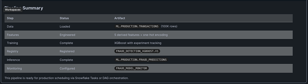
The Full Pipeline Summary
| Stage      | Artefact                        | Notes                                                               |
| ---------- | ------------------------------- | ------------------------------------------------------------------- |
| Data       | ML.PRODUCTION.TRANSACTIONS      | 100K+ rows, ~1% fraud rate                                          |
| Features   | Derived + One-Hot Encoded       | RISK_COMPOSITE, LOG_AMOUNT, ratio/hour features                     |
| Training   | XGBoost                         | scale_pos_weight, aucpr optimised, early stopping at best iteration |
| Registry   | FRAUD_DETECTION_XGBOOST.V1      | Metrics attached, schema inferred from sample input                 |
| Inference  | ML.PRODUCTION.FRAUD_PREDICTIONS | Column-aligned, threshold-applied, SCORED_AT stamped                |
| Monitoring | FRAUD_MODEL_MONITOR             | Daily refresh, score distribution + drift tracking                  |
This pipeline is ready to be wrapped in a Snowflake Task or DAG for scheduled production runs — no external orchestration required.
What Snowflake’s Agentic ML Layer Adds
If you’ve been following Snowflake’s ML roadmap, Cortex Code — now generally available — can generate pipelines like this from natural language prompts. Snowflake has shared results from First National Bank of Omaha using Cortex Code for forecasting and anomaly detection, reporting a 10x productivity gain. That’s not a claim about replacing data scientists; it’s a claim about eliminating the scaffolding work that consumes most of their time.
The pipeline above is what you’d produce working manually — and it’s a solid, production-ready foundation. Cortex Code accelerates the path to that foundation by handling documentation lookup, boilerplate debugging, and hyperparameter reasoning. Either way, the destination is the same: a governed, versioned, monitored model running next to your data inside Snowflake.
Key Takeaways for Practitioners
Keep your feature engineering deterministic. The same transformation logic must run identically at training time and inference time. If it diverges — even by a rounding rule or a category that appears in one dataset but not the other — you get silent degradation, not loud errors.
Optimise for the right metric. On imbalanced fraud data, accuracy is a lie. Average Precision, F1 at your operating threshold, and the shape of the precision-recall curve are your real benchmarks.
Register everything. A model that lives only in a notebook is one laptop failure away from being lost. The Snowflake Model Registry gives you versioning, lineage, and the ability to call models by name from any Snowpark session.
Monitor before you need to. Set up drift checks when you deploy, not when someone notices the fraud rate has inexplicably doubled. FRAUD_MODEL_MONITOR costs almost nothing to run; the alternative costs a lot more.
Enjoyed this article?
👏 Give it a clap if it added value
🔗 Share it with your team — fraud detection is a team sport, not a solo project
➕ Follow for more deep-dives on Snowflake, data engineering, and cloud architecture
📍 Find me here: Medium: @SnowflakeChronicles
LinkedIn: satishkumar-snowflake
#Snowflake #SnowflakeML #MachineLearning #FraudDetection #DataEngineering #XGBoost #MLOps #CortexAI #CloudDataPlatform #SnowflakeChronicles #DataScience #FeatureEngineering #ModelRegistry #MLObservability #Snowpark
Building a Production-Grade Fraud Detection Pipeline Inside Snowflake — End to End was originally published in Towards AI on Medium, where people are continuing the conversation by highlighting and responding to this story.