
In the previous article, we saw why early neural language models mattered. They moved language modeling beyond pure counting and into learned prediction. They showed that a model did not have to live only by frequency tables and exact fragment matches. It could learn internal representations and use them to make better guesses.
But that still leaves an important gap in understanding.
It is one thing to say that a model uses embeddings, learned weights, and a hidden layer. It is another to see, clearly and concretely, what each of those pieces is doing.
This article is about that second task.
Here, we are not mainly asking why the field moved beyond n-grams. We are asking what an early neural language model actually looks like from the inside. What is the world it lives in? What does its training data look like? What is a word identity? What is an embedding? What exactly enters the network? What does the hidden layer do? What comes out? And how does repeated correction gradually turn context into prediction?
In other words, this is not another historical introduction. It is a closer look inside the first neural language model itself. And that matters because once the machine becomes clear, the next architectural leap — recurrence — stops feeling magical. It begins to feel necessary.

A quick bridge from Series A
By the end of Series A, we already understand a crucial idea: words do not have to remain isolated labels. They can be represented as dense vectors, and words that behave similarly can end up near one another in a learned space.
That idea matters enormously. It gives a model a way to treat related words as related, instead of as completely separate symbols. But a word vector by itself is not yet a prediction.
A vector is a representation, not a continuation. It can tell us something about how a word behaves, but not yet what word should come next in a sentence. So the real question now is no longer whether neural language models were a breakthrough. The real question is how that breakthrough actually works from the inside.
Historically, early neural language models were among the first places where distributed word representations were learned and used inside a predictive system. In other words, the model did not just learn word vectors in isolation; it learned how to use a short visible context of such vectors to produce a next-word prediction.
So this article is not reintroducing the neural turn. It is opening that early neural language model and examining its internal pipeline.
Before we draw the network, we need a small world
A real language model may know tens of thousands of words, or far more. But that is too large to hold clearly in the mind at first. So to understand the basic idea, it helps to shrink the world.
Let us imagine a tiny vocabulary of just ten words:
the, cat, dog, puppy, fox, sat, ran, slept, on, mat
Now the task becomes easier to picture.
If the model is asked to predict the next word, it is not choosing from all of language. It is choosing from these ten known possibilities. That means the output side of the model can be imagined as producing one score for each of those ten words.
So if the current context is: the cat
then the model is really asking:
Among these ten words, which one should come next?
That smallness matters.
It makes the architecture visible.
It lets us see what prediction means before the scale of real language makes everything abstract.
A real language model’s world is far larger. But for understanding the mechanism, a small world is a gift.
What the training data actually looks like
Once the vocabulary is fixed, the training data becomes much easier to picture. A language model is not trained on isolated words floating in space. It is trained on sequences made from the words in its world. In our tiny example, suppose the model’s vocabulary is:
the, cat, dog, puppy, fox, sat, ran, slept, on, mat
Then a toy training corpus might contain short sequences like these:
the cat sat
the dog ran
the puppy slept
the fox sat
the cat sat on the mat
.
.
.
the dog slept on the mat
These full sequences are the raw material. But they are still not the final objects that the network trains on. The model does not swallow an entire sentence in one gulp and directly “understand” it. Instead, the sentence is broken into many smaller training examples.
Suppose the visible context window is two words wide. Then each position in a sentence can become a little prediction task.
Take the sequence: the cat sat
From this, we can cut the training example:
context: the cat target: sat
That means the model is shown the context the cat, and the desired next word for that example is sat.
Now take the longer sequence: the cat sat on the mat
This does not produce just one example. It produces several:
context: the cat target: sat
context: cat sat target: on
context: sat on target: the
context: on the target: mat
So one sentence becomes multiple context → next-word training pairs. That is a very important point. The training corpus is made of sequences. The actual training process is made of many smaller supervised prediction examples cut out of those sequences. If the context window were three words wide instead of two, then the examples would change.
From: the cat sat on the mat
we would get things like:
context: the cat sat target: on
context: cat sat on target: the
context: sat on the target: mat
So the window size determines how much of the recent past the model is allowed to see when making each prediction.
This is also why the training data and the vocabulary play two different roles.
The vocabulary tells the model what words exist in its world and what words it is allowed to predict.
The training corpus tells the model which sequences actually occur in that world.
And the training examples are the little context → target pairs extracted from those sequences.
That three-level distinction helps a lot:
vocabulary = what words exist
corpus = what sentences or sequences exist
training examples = what local prediction tasks are cut from those sequences
Once that is clear, many other parts of the model become easier to understand.
For example, when we later say that the model is trained to make the “correct” next word more likely, we do not mean correct in some absolute or eternal sense. We mean correct for this particular training example.
After the cat, many continuations might be plausible in natural language. sat could be plausible. ran could also be plausible in a different sentence. But if the current training example comes from the sequence the cat sat, then for that step the target is sat.
So the model is always learning from a local supervision signal supplied by the corpus. That is the immediate world it inhabits during training. Another subtle point also becomes visible here.
Because the model sees many overlapping examples, it does not just memorize one sentence at a time. From repeated exposure, it begins to notice regularities across many training pairs:
after the cat, certain kinds of words often appear
after sat on, some nouns become more likely
after on the, location-like or object-like words may follow
This is exactly where learning begins to move beyond raw lookup. The network is not merely storing one phrase after another in isolation. It is being exposed to many small predictive situations, and its parameters gradually adjust so that similar contexts can produce similar expectations.
So the training data is not just “a lot of text.” It is text turned into a large collection of little prediction problems.
And that is what makes next-word prediction such a powerful organizing task. A corpus of sentences becomes a stream of supervision. Every short stretch of text becomes a chance for the model to ask: given these words, what should come next? That is the form in which language enters the neural model.
In real training systems, a few extra practical details are usually added around this basic setup. Special tokens often mark the beginning of a sequence and the end of a sequence — commonly written as BOS and EOS. These matter because otherwise the model would only learn to keep predicting the next word without any explicit notion of where a sentence begins or where it should stop. If the model sees BOS the cat sat EOS, then learning includes not only that sat may follow the cat, but also that after the final word the correct continuation may be EOS, meaning the sequence should end.
When many training examples are processed together, they are usually grouped into batches so the model can learn efficiently in parallel. But different sequences often have different lengths, so shorter ones may be extended with padding tokens just to make the batch rectangular and easier to process computationally. These padded positions are typically treated as structural placeholders rather than meaningful language targets. So while BOS, EOS, padding, and batching belong to the engineering side of training, they still serve the same central idea: a corpus is turned into many small next-word prediction tasks, with explicit markers for where sequences start, where they stop, and how many examples can be trained together.

A word begins as an identity
Now that we have shrunk the world to a small vocabulary, we can look more closely at what a word is inside the model.
Before a word becomes a rich learned vector, it begins in a simpler form: as an identity inside the vocabulary.
If the model’s world is:
the, cat, dog, puppy, fox, sat, ran, slept, on, mat
then each word must first have a place in that list. In that sense, the model initially needs to know not what the word means, but simply which word it is.
One blunt way to represent that identity is with a one-hot vector.
So if dog is the third word in the vocabulary, we can represent it like this:
[ 0, 0, 1, 0, 0, 0, 0, 0, 0, 0 ]
That vector is extremely simple. It tells the model one thing and one thing only:
this is dog
But that is also its limitation.
It does not say that dog is similar to puppy.
It does not say that cat is also an animal.
It does not say that sat and slept might behave similarly in some contexts.
A one-hot vector is identity without geometry.
It tells us which word, but not how that word relates to other words.
So if language modeling stayed at this level, it would remain trapped inside discrete symbols. The model would know how to distinguish words, but not how to place them in any meaningful relation to one another.
That is exactly why embeddings matter.
From identity to embedding
Instead of using the one-hot identity as the model’s main working representation, neural language models learn something denser and more expressive for each word. That learned object is the embedding.
So the progression is:
word
→ vocabulary identity
→ embedding vector
This distinction matters.
A one-hot representation tells the model only which word it is.
An embedding begins to tell the model how that word behaves.
And because embeddings are learned from data, words that occur in similar kinds of contexts can gradually end up near one another in the learned space.
That is how dog and puppy can begin to resemble one another inside the model.
Not because anyone manually declared that similarity in advance.
But because training repeatedly rewards the model when words that behave similarly are treated in similar ways.
If dog and puppy often appear in related environments and support related predictions, then it helps the model if their embeddings become somewhat alike. So over time, learning pushes them toward nearby regions of the space.
That is one of the deepest differences between count-based models and neural ones. Count-based models mainly remember fragments. Neural models can learn a shared representational space. And that shared space is what makes softer, more flexible generalization possible.

A gentler way to picture a neural network
The phrase neural network often sounds more intimidating than it needs to. So let us not begin with formulas. Let us begin with a picture.
Imagine a machine with many little knobs inside it.
You feed an input into the machine. Because of how those knobs are currently set, the machine produces some output. Then you compare that output with the correct answer. If the machine was off, you turn the knobs slightly.
Then you try another example. And another. And another.
Over time, after seeing many examples and being corrected many times, the machine gradually settles into better internal settings. It becomes more skillful at turning certain kinds of inputs into useful outputs.
That is the simplest honest picture of a neural network.
It is a model with many adjustable internal settings. Learning means tuning those settings through repeated examples.
In more formal language, those internal settings are called weights. But it is better to feel the idea first.
The network is not memorizing every case separately like a dictionary of isolated fragments. It is learning how to set its internal knobs so that certain kinds of inputs tend to produce better outputs.
That is the shift.
A count table stores observed frequencies.
A neural network learns an internal configuration.
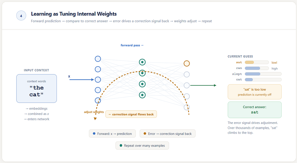
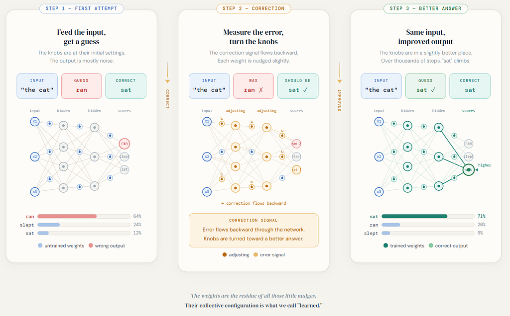
What learning means here
Suppose the model sees the short context: the cat
And suppose that, in one training example, the next word is: sat
At first, the model may not be very good. Its internal settings are not yet well tuned. It may give too much importance to irrelevant words and too little to sat. But then the model is shown the mistake.
So its internal settings are adjusted slightly in the direction that would have made sat more likely. Then another example comes.
Maybe: the dog → ran
Again the internal settings are adjusted. Not so that only this one case is memorized, but so that the whole machine becomes a little better at mapping short contexts to likely next words. After many examples, the network gradually begins to discover useful regularities.
Some contexts begin to pull the output toward verbs.
Some contexts begin to favor nouns.
Some begin to activate certain patterns of continuation more than others.
That is what it means for the model to learn. It is not handed a finished list of rules. It is tuned.
And through that tuning, context gradually becomes something the machine can transform into prediction. One subtle clarification matters here.
When we say correct, we do not mean universally correct for all imaginable language. After the cat, both sat and ran could be plausible in different sentences. But during training, the model is shown one specific example from the dataset, and for that example the “correct” next word is whatever the data provides.
If the training example is: the cat sat
then the model is nudged toward sat for that learning step.
So the training data defines the model’s immediate world: not all possible truths, but the particular statistical world represented by the examples it has been given.
How embeddings are actually fed into the network
This is the point where the machinery must become explicit. Suppose the visible context is: the cat
Each word in that context is already available as an embedding. So the model now has:
e(the)
e(cat)
These are dense numeric vectors.
The model then combines them into a single input vector. In many early neural language models, the common choice was concatenation: place the vectors side by side.
So the combined input becomes:
x = [e(the); e(cat)]
That combined vector x is what enters the neural network. This matters.
The network does not consume raw words directly. It consumes the numeric coordinates of their embeddings, combined into one input vector for the visible context window.
That means the input side of the main neural network is not “one neuron per vocabulary word.” It is “one coordinate per component of x.”
The output side, however, does return to vocabulary space.
The network produces one score for each possible next word in the vocabulary, and those scores can then be turned into probabilities.
So the structure is:
context words
→ embeddings
→ combined vector x
→ hidden layer
→ output scores over vocabulary
→ probabilities
That is the real pipeline.

The same pipeline, opened up more carefully
It is easy to say:
Take the context words, turn them into embeddings, join them into x, pass x through the network, get vocabulary scores.
That is enough to understand the flow. But it still hides an important question: what exactly is the network touching?
This is where a more detailed diagram becomes useful.
Raw words like the and cat do not themselves enter the network as words. Each word is first identified in the vocabulary, mapped to a dense embedding, and then those embeddings are flattened into one longer numeric vector.
If each embedding had 4 numbers, then two embeddings together would produce an 8-number input vector. It is those 8 numbers that feed the input layer.
So the input neurons are not the, cat, or other vocabulary words. They are simply the coordinates of x.
The output side is different. There, each output neuron does correspond to one possible next word in the vocabulary. After softmax, those scores become probabilities.
That distinction is one of the most important pieces of clarity in the whole model:
input side: coordinates of the combined context vector
output side: scores over the vocabulary
Once that becomes clear, the rest of the network becomes much less mysterious.


How one prediction becomes a sequence
A language model does not generate a sentence all at once. It generates by repetition.
At one moment, it sees a short visible context and predicts a likely next word. That word is then added to the text. The visible window shifts forward, and the same model is asked again.
So if the current context is: the cat
The model might produce: sat
Now the text has grown to: the cat sat
Window size is 2 word wide, the model now looks only at: cat sat
and predicts again — perhaps: on
Now the text becomes: the cat sat on
Then the window shifts once more to: sat on
and the next prediction might be: mat
So even a fixed-window neural language model can still generate a flowing sequence:
the cat → sat
cat sat → on
sat on → mat

That is how one-step prediction becomes multi-step generation. But notice what has not happened. The model is not carrying a rich internal memory of the whole sentence. It is simply being reused on a sliding local window.
The sentence grows, but the model’s immediate field of view remains narrow. That difference matters. It is exactly what later sequence models try to overcome.
The hidden layer, without the drama
Inside the network, the input does not usually go straight to the output. It first passes through an internal representation.
This is often called a hidden layer.
The name sounds more mysterious than it is. It simply means a layer inside the model that is neither the raw input nor the final output. It is an internal stage of processing.
Why is that useful?
Because it gives the model room to reshape the context before making its prediction. Instead of jumping directly from the visible words to next-word scores, the network can first build its own internal representation of the context.
That internal representation may capture things that help prediction:
some rough sense of grammatical pattern
some rough sense of word compatibility
some rough sense of what kinds of words tend to follow what kinds of contexts
Not in a neat human-readable way. But in a learned internal way.
It is not a vocabulary layer and not a memory bank of exact words. It is a learned intermediate representation of the visible context.
This is one of the deepest shifts in early neural language models.
The model is no longer merely storing what followed what.
It is building an internal state of processing from which prediction can emerge.
That is why this stage matters so much. Language modeling has begun to acquire an inner layer.
A small example of why this felt different
Suppose a count-based model has seen:
the dog ran
the cat slept
the fox sat
Now suppose it sees:
the puppy
If the puppy was rare in the data, a count-based model may not know much. It wants direct support from exact frequency.
A neural model may still struggle, but it has a better kind of chance.
Why?
Because puppy is represented by an embedding, and that embedding may occupy a region of the learned space that behaves somewhat like other animal-related or noun-like words the model has already encountered. The model does not need to have seen the exact phrase many times in order to make a more informed guess. Its learned internal settings may already know something about how contexts like:
the dog
the cat
the fox
tend to continue.
So the model is no longer only asking:
Have I seen this exact fragment enough times?
It is beginning to ask:
What does this context resemble?
That is a much more powerful habit of mind.

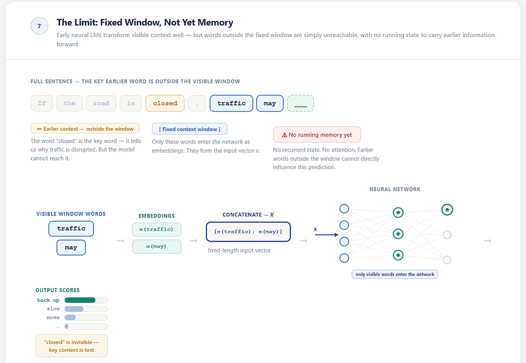
But the window was still fixed
For all their progress, these early neural language models still worked through a fixed context window.
In the examples here, the visible context window is two tokens long. But the same idea holds for three words, or four, or more.
The model always sees only a chosen local block. Those words are turned into embeddings, combined into one input, and passed through the network.
That was richer than n-grams in an important way. The model was no longer only counting; it was learning. But structurally, it was still trapped inside a bounded frame.
Only the visible context could influence the current prediction.
If something important had happened earlier — outside the chosen window — then the model had no real place to keep it.
That is why this stage, for all its beauty, was still incomplete.
The model had learned how to transform a short context.
It had not yet learned how to carry context forward through time.
That is the difference.
A fixed-window neural model becomes better at processing the visible slice.
A recurrent model will later try to preserve a running trace of the past itself.
That is the next leap.
Why this stage still mattered enormously
It would be easy, knowing what came later, to rush through this stage and treat it only as a prelude.
That would be unfair. Because this stage changed the nature of the model.
Before this, prediction was still mostly tied to counted local fragments. After this, the model had begun to develop an internal computational life. It could take a visible context, reshape it through learned settings, build an internal representation, and produce a prediction from that internal processing.
That is not a small change. It is the step that made later architectures possible.
Without this stage, there would be no meaningful way to talk about hidden representations, learned internal features, or networks discovering useful structure inside language. The field first had to move from stored frequency to learned transformation.
That is what early neural language models gave us. They taught the model how to compute with context.
The question they left behind
And yet their limitation was clear enough that the next question almost asks itself.
If a model can learn how to transform the visible context into a prediction, can it also learn how to keep some trace of earlier context alive as language unfolds?
Can it stop rebuilding everything from a fixed window each time?
Can it carry something forward?
That question leads directly to recurrent neural networks. And that is where the story goes next.
One-line memory hook
Early neural language models stopped just counting short contexts and started learning how to transform them — but they still saw language through a fixed window.
Inside an Early Neural Language Model: Vocabulary, Embeddings, Training and Prediction was originally published in Towards AI on Medium, where people are continuing the conversation by highlighting and responding to this story.