Written quickly for the Inkhaven Residency.[1]
There’s a phenomenon I often see amongst more junior researchers that I call being scared of math.[2] That is, when they try to read a machine learning paper and run into a section with mathematical notation, their minds seem to immediately bounce off the section. Some skip ahead to future sections, some give up on understanding the section immediately, and others even abandon the entire paper.
I think this is very understandable. Mathematical notation is often overused in machine learning papers, and can often obscure more than it illuminates. And sometimes, machine learning papers (especially theory papers) do feature graduate level mathematics that can be hard to understand without knowing the relevant subjects.
Oftentimes, non-theory machine learning papers use mathematical notation in one of two lightweight ways: either as a form of shorthand or to add precision to a discussion.
The shorthand case requires almost no mathematical knowledge to understand: paper authors often use math because a mathematical symbol takes up far less real estate. As an example, in a paper about reinforcement learning from human preferences, instead of repeating the English words “generative policy” and “reward model” throughout a paper, we might say something like “consider a generative policy G and a reward model R”. Then, we can use G and R in the rest of the paper, instead of having to repeat “generative policy” and “reward model”. This is especially useful when trying to compose multiple concepts together: instead of writing “the expected assessed reward according to the reward model of outputs from the generative policy on a given input prompt”, we could write E[R(G(p))].
Similarly, mathematical notation can be used to add precision to a discussion. For example, we might write R : P x A -> [0,1] to indicate the input-output behavior of the reward model. This lets us compactly express that we’re assuming the reward model gets to see both the actions taken by the policy (A) and the prompt provided to the policy (P), and that the reward it outputs takes on values between 0 and 1.
In neither case does the notation fundamentally depend on knowing lots of theorems or having a mastery of particular mathematical techniques. Insofar as these are the common use cases for mathematical notation in ML papers, sections containing the math can be deciphered without having deep levels of declarative or procedural mathematical know-how.
What to do about this
I think there are two approaches that help a lot when it comes to overcoming fear of math: 1) translating the math to English, and 2) making up concrete examples.
As an illustration, let’s work through the first part of section 3.1 of the Kalai et al. paper, “Why Language Models Hallucinate”. I’ll alternate between two moves: restating each formal step in plain English, and instantiating it with a deliberately silly running example:
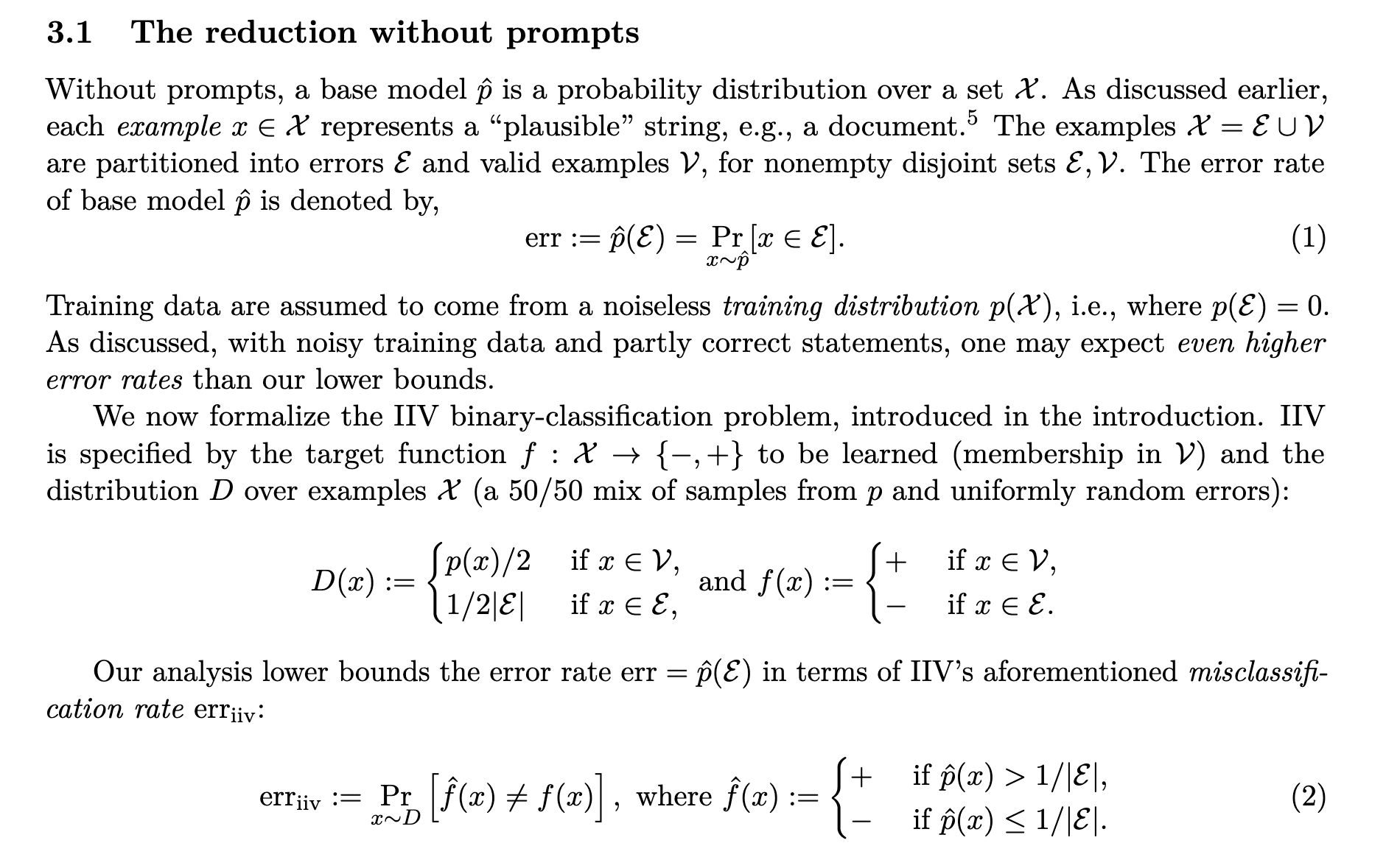
The section starts by saying that a base model can be thought of as a probability distribution over a set of possible strings (“examples”) X. As an example, a model such as GPT-2 can indeed be thought of as producing a probability distribution over sequences of tokens of varying length.[3]
Then, the authors write that these possible strings can be considered as errors or valid examples, where each string is either an error or valid example (but not both). Also, the set of example strings include at least one error and one valid example. The training distribution is assumed to include only valid examples.
Here, it’s worth noting that an “error” need not be a factually incorrect statement, nor that the training distribution necessarily includes all valid statements. Let's make up a rather silly example which is not ruled out by the authors’ axioms: let the set of plausible strings be the set of English words in the Oxford English dictionary, let the set of “valid” strings be the set of all words with an odd number of letters, while the training distribution consists of the single string “a” (p(x) = 1 if x = “a” and 0 otherwise).
The authors now formalize the is-it-valid (IIV) binary classification problem. Specifically, the goal is to learn the function that classifies the set of all strings into valid examples and errors. In our case, the function is the function that takes as input any single English word, and outputs 1 if the number of letters in the word is odd. Also, we evaluate how well we’ve learned this function on a distribution that’s a 50/50 mixture of strings in the training distribution (that is, the string “a”) and the strings that are errors, sampled uniformly (that is, all English words with an even number of letters.)
The authors then introduce the key idea: they relate the probability of their learned base model to its accuracy as a classifier for the IIV problem. Specifically, they convert the probability assigned by the base model to a classification: if it assigns more than 1/number of errors probability to a string, then the base model classifies the string as a valid string. Otherwise, it considers it an error.
The authors then introduce their main result, which relates the error of this IIV classifier to the probability the base model generates an “erroneous” string:
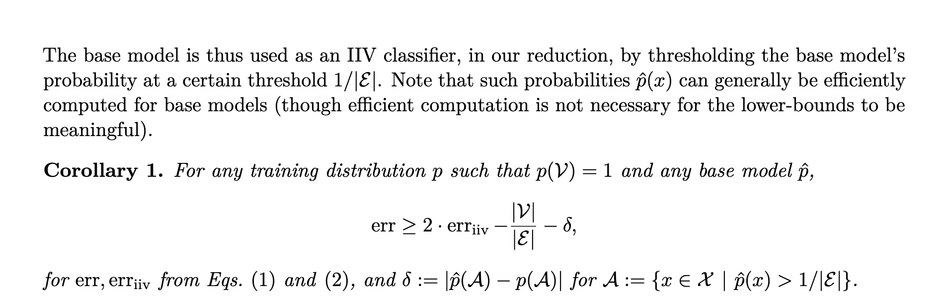
That is, the probability our base model generates an erroneous string is at least twice the error rate of the converted classifier on the IIV classification problem, minus some additional terms relating to the size of the valid and error string sets and the maximal difference between the probability assigned to any string by the training distribution and the base model.
To make sure we understand, let’s continue making up our silly example: our base model assigned 50% probability to the string “a” and 50% to “b” (and 0% to all other strings). Then (since it assigns 0% probability to any string with an even number of letters), its classification accuracy on the IIV problem is 100%, and its error rate is 0%. Indeed, the probability it generates an erroneous string is 0%. So we actually already have err = 0 >= 2 * err_iv = 0, trivially. It’s worth checking what the other terms here are, to make sure we understand: the first term is the ratio of the size of the set of valid strings and the set of erroneous string (in our case, the ratio of the number of English words with odd characters versus even ones), and the second is 0.5 – our base model assigns a 50% chance to “a”, which the training distribution assigns 100% probability to, and similarly our base model assigns a 50% chance to “b”, which the training distribution assigns 0% chance to.
I’m going to stop here, but I hope that this example shows that math is not actually that hard to read. Most non-theory ML papers have math sections that are similar in difficulty to this example. If you find yourself bouncing off the math, the question is rarely "do I know enough math for this?", and much more often "how can I translate this to English and use an toy illustrative example to make it concrete?"
- ^
I was going to conclude my “have we already lost” series, but I wanted to write about something lighter and less serious for a change.
- ^
There’s also a more general phenomenon that I’d probably call being scared of papers, to which the only real solution I’ve found is exposure therapy (interestingly, writing a paper does not seem to fix it!).
- ^
Specifically, GPT-2 takes as input a sequence of tokens, and assigns a probability distribution over 50,257 possible next tokens, one of which is the <|endoftext|> token. Starting from the empty sequence, GPT-2 induces a probability distribution over token sequences of any length, by multiplying the conditional probabilities of each subsequent token in the sequence, conditioned on all previous tokens.
Discuss