How LLMs reuse history, read memory, and transform computation into data movement

In the previous article, we saw that LLM inference slows down as context grows.
Not just because there is more computation,
but because the system itself shifts from being compute-bound to memory-bound.
That raises a natural question.
If memory access is now the bottleneck,
what does that actually look like inside the model?
What is the system doing at each step, and why does the cost keep growing?
From the outside, this process looks simple.
You send a prompt.
The model responds.
But internally, the system is not doing one kind of work.
It switches between two very different modes of execution, each with its own cost and constraints.
Understanding that shift is key to understanding inference.
A Single Request, Two Very Different Phases
When you send a prompt to an LLM, the model does not process it in a single uniform way.
Instead, inference unfolds in two distinct phases:
In the first phase, prefill, the model processes the entire prompt.
In the second phase, decode, it generates one token at a time.
At a high level, both phases use the same model and the same attention mechanism.
But how that computation is executed is fundamentally different.
This difference in structure is what drives the transition from compute-bound to memory-bound behavior, from efficient parallel computation to repeated, sequential memory access.
To see why these phases behave so differently, we need to examine how the computation is structured in each one.
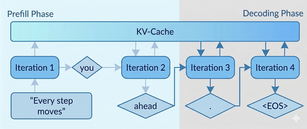
Prefill: One Large, Parallel Computation
The first phase is prefill.
The model takes the entire prompt and processes it in a single forward pass, with all tokens fed in together and attention computed across the full sequence.
Because everything is available upfront, the model can perform these computations in parallel.
This is exactly the kind of workload GPUs are designed for: thousands of cores executing the same operations simultaneously, over large blocks of data.
To make this concrete, consider a prompt with 1000 tokens.
During prefill, the model processes all 1000 tokens in a single pass.
Each token attends to the others, and the full set of Keys and Values is computed for every layer.
For a model with 32 layers and a hidden dimension of 4096,
this means computing and temporarily holding millions of values in GPU memory, all at once, before a single output token is produced.
In practice, this work can dominate total latency for long prompts.
The user is already waiting, and the model has not generated a single word of response yet.
But this computation is structured in a way that allows the GPU to operate efficiently. The operations are large, dense, and parallel, which keeps the GPU fully occupied.
At this stage,
the system is still dominated by computation, and adding more compute can still improve performance.
At the end of this phase, the model has built up a complete set of Keys and Values for the entire prompt.
These Keys and Values do not disappear after prefill.
They become the foundation for everything that happens during generation.
But prefill only processes what you gave the model.
The harder problem begins when it starts generating what comes next.
Decode: One Token at a Time
Once the model finishes processing the prompt, it enters the decode phase.
This is where it begins generating new tokens.
Unlike prefill, this phase is not a single, large computation.
It is a loop.
At each step, the model generates one token,
appends it to the sequence,
and then uses the entire accumulated context to produce the next one.
To see what this means in practice, consider the same 1000-token prompt.
To generate the first new token,
the model attends over all 1000 tokens.
To generate the second, it attends over 1001 tokens.
Then 1002.
Then 1003.
Nothing about the earlier tokens has changed.
But they are still used again at every step.
Each token also depends on the one before it.
The model cannot know what to generate at step two until step one is complete.
This sequential dependency means the GPU, which is built for parallel workloads, is now processing one small operation at a time, a fraction of its actual capacity.
Instead of one large, efficient computation, the system now performs many smaller computations, one per token, each over a slightly larger context than the last.
For example, generating the 500th token requires attending over roughly 1500 tokens, assuming a 1000-token prompt.
Generating the 1000th requires attending over roughly 2000 tokens.
That information does not need to be recomputed.
But it does need to be loaded from memory, again and again, at every single step.
So each step increasingly becomes a problem of data access rather than computation.
Prefill is primarily a throughput problem, processing as much data as possible at once.
Decode is a latency problem, where each step must complete before the next begins.
If the context does not change between steps, why is the model using it again every single time?
KV Cache: Avoiding Recomputation
In a naive implementation, the model would recompute everything at every step.
To generate the next token, it would process the entire sequence again,
recompute all Keys and Values, and run attention from scratch.
This quickly becomes prohibitively expensive.
For a longer sequence, each new token requires redoing nearly the same computation over an almost identical context.
Most of that work is repeated, with only a single new token added each time.
Modern systems avoid this with a straightforward optimization.
Store the past.
Instead of recomputing Keys and Values for every token at every step,
the model computes them once during prefill, and stores them in memory.
This stored representation is the KV cache.
When generating new tokens, the model reuses these stored Keys and Values, and only computes what is new.
So instead of rebuilding the entire history, the model extends it.

KV cache removes redundant computation. But it does not remove the dependency on the past.
The cost does not disappear. It moves.
From computation to memory.
And that shift is what defines how modern inference systems behave.
What KV Cache Actually Stores
To understand why KV cache becomes a problem, we need to look at what is actually being stored.
At every layer of the model, each token produces two vectors: a Key and a Value.
These vectors are not small.
They have the same hidden dimension as the model, often thousands of numbers per token.
During prefill, the model computes these Keys and Values for every token in the prompt, across every layer.
KV cache stores all of them.
To make this concrete, consider a model with 32 layers and a hidden dimension of 4096.
For a single token, this means storing a Key and a Value vector at each layer.
That is: 2 × 4096 × 32 = 262,144 values per token.
In FP16, each value takes 2 bytes.
So a single token requires roughly 512 KB of memory across the full model.
For a sequence of 10,000 tokens, that grows to around 5 GB of memory.
And this is just for one request.
In practice, this representation is split across multiple parallel attention components, each maintaining its own Keys and Values, increasing the overall memory footprint.
As the model generates more tokens, the cache keeps growing.
Every new token adds its own Keys and Values, across every layer.
So the memory usage grows linearly with sequence length.
At larger context sizes, a single request can consume tens of gigabytes of GPU memory.
And unlike prefill, this memory is not temporary.
It must remain available for every subsequent step in decode.
The model is no longer just computing over the sequence.
It is carrying the entire history with it.
The Real Bottleneck: Memory Access
KV cache removes redundant computation. But it replaces it with something else.
Repeated access to memory.
At every step in decode, the model must read all previously stored Keys and Values from memory, use them once for attention, and then repeat the process for the next token.
Nothing about that data changes.
But it still needs to be loaded again, step after step.
This is where memory bandwidth becomes the limiting factor.
During prefill, the workload is dominated by large, dense computations.
These operations keep the GPU fully utilized, performing a large amount of computation for every byte of data moved.
During decode, that balance shifts.
Each step involves relatively little computation, but requires accessing a large and growing amount of data.
The GPU is no longer limited by how fast it can compute.
It is limited by how fast it can move data.
This is what it means for a system to be memory-bound.
Each new token requires scanning a larger history, which increases the amount of data that must be read.
So even though the model is doing less computation per step, latency continues to increase.
And because these steps are sequential, this delay cannot be hidden through parallelism.
This is the fundamental constraint of modern LLM inference.
Not just computation, but data movement.
And once you see that, the next question becomes unavoidable.
If memory access is the bottleneck,
how do modern systems store, organize, and retrieve this data efficiently?
Reducing KV Size: MQA and GQA
By this point, the bottleneck is clear.
Each decode step depends on the entire KV cache, and that cache grows with every token.
If we cannot avoid reading everything that came before, the next question becomes:
Can we make that representation smaller?
We saw earlier that storing Keys and Values costs roughly 512 KB per token,
or around 5 GB for a 10,000-token sequence.
So the problem is not just that we store history. It is how much we store per token.
To understand where that cost comes from, we need to look at how attention is structured.
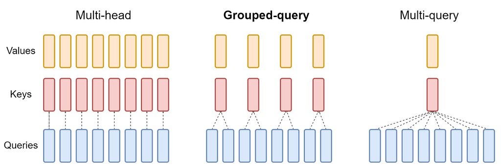
A transformer does not rely on a single attention mechanism. Instead, it uses multiple parallel attention heads.
Each head looks at the same sequence, but learns to focus on different relationships.
One head might capture syntax, another might capture long-range dependencies, another might track entities.
This allows the model to capture different types of relationships within the same sequence.
But there is a cost.
Each attention head maintains its own Keys and Values.
So for every token, we are not storing one representation, but many.
For example, if a model has 32 attention heads, then each token contributes 32 separate KV sets.
That is what causes the KV cache to grow so quickly.
This is where Multi-Query Attention (MQA) comes in.
Instead of storing separate Keys and Values for each attention head, MQA shares a single set of Keys and Values across all heads.
Each head still computes its own Query at every step. Unlike Keys and Values, Queries are not reused. They are generated from the current token,
and represent what the model is looking for at that moment.
This dramatically reduces the KV cache.
What was previously 32 KV sets per token becomes just 1.
That is where the reduction comes from.
For the same 10,000-token sequence, what was roughly 5 GB of KV data drops to around 150 MB.
And more importantly, each decode step now requires reading far less data from memory.
But this simplicity comes with a real tradeoff.
If all attention heads see the same Keys and Values, they lose the ability to specialize.
They are no longer looking at the sequence from different perspectives.
In practice, this can limit the model’s ability to capture complex relationships, which is why full MQA is rarely used in large models.
So instead of full sharing, modern systems use Grouped Query Attention (GQA).
Here, attention heads are divided into smaller groups.
For example, 32 heads might be split into 4 groups.
Heads within a group share Keys and Values, but different groups maintain their own.
So instead of one KV set per head, or one KV set for the entire model, we have one KV set per group.
That means 32 KV sets become 4, which reduces the KV cache by a factor of 8.
For the same 10,000-token sequence, what was roughly 5 GB now becomes:
5 GB ÷ 8 ≈ 625 MB.
This reduces the KV cache significantly, while still preserving some diversity in how the model attends to the sequence.
And more importantly, it reduces how much data must be read at every decode step.
At this point, the goal is no longer just to compute efficiently.
It is to reduce how much information must be moved.
Because in decode, performance is determined not by how fast we compute, but by how little we need to read.
Putting It All Together
What we have seen so far is a pattern.
Every optimization in LLM inference does not remove a cost.
It moves it.
From large parallel computation, to repeated memory access, to managing how that memory grows over time.
And that shift changes what it means to make inference efficient.
It is no longer just about faster kernels or more compute.
It is about deciding what to store, what to evict, and what to reuse across steps.
Because in decode, performance is determined not by how fast we compute, but by how little we need to read.
That is why techniques like MQA and GQA matter.
They reduce duplication in the KV cache.
But they do not solve the problem.
They only delay it.
As sequences grow, the KV cache still expands, and memory remains the limiting factor.
So the next question is not just how to reduce it.
It is how to manage it when it no longer fits cleanly in memory.
That is where techniques like PagedAttention, radix-based prefix sharing,
prefill caching, and other memory-management strategies enter the picture,
each designed to handle a different aspect of the same constraint: how to keep an ever-growing KV cache usable in practice.
That is the next layer of the story. If you found it useful, follow along. The next part is where the system gets really interesting to think about.
Inside LLM Inference: KV Cache, Prefill, and the Decode Bottleneck was originally published in Towards AI on Medium, where people are continuing the conversation by highlighting and responding to this story.