Originally published on LinkedIn
What happened when we deployed a real VQC on EEG brain data and what four experiments actually told us about where quantum ML stands today.
Quantum machine learning is one of those fields where the gap between theory and honest experimental evidence is wider than most people admit.
This is an attempt to close that gap at least for one specific problem, one specific circuit, and four specific experiments that didn’t go the way the theory suggested they would.
Spent the last few years working at the sharp end of post-quantum cryptography building systems, running formal verification, writing code that has to work in production under real conditions. When the opportunity came up to apply quantum machine learning to “ADHD focus detection from EEG brain signals”, it was too interesting to pass up.
Four experiments. Real data. Every number published including the uncomfortable ones.
The biological foundation
The human brain generates electrical oscillations across five distinct frequency bands simultaneously. These aren’t metaphors, they’re measurable voltage fluctuations across the scalp, each carrying different information about cognitive state:
- Delta (1–4 Hz) — deep sleep, physical recovery
- Theta (4–8 Hz) — drowsiness, mind-wandering, attentional drift
- Alpha (8–13 Hz) — relaxed alertness, calm wakefulness
- Beta (13–30 Hz) — active cognitive engagement, task focus
- Gamma (30–50 Hz) — high-level processing, perceptual binding
When attentional focus collapses, the shift is measurable before the individual consciously registers it. Theta power rises. Beta power drops. The ratio between them — computed across both Beta sub-bands — becomes the primary signal:
FocusRatio = Theta / (Beta1 + Beta2)
This ratio, alongside the eight individual band-power features, forms the complete 9-dimensional input to the classifier. The research question: can a quantum circuit learn to separate high-focus states from lapse states using this feature set — and does it do so better than a classical model operating on the same inputs?
Why the quantum approach is theoretically motivated
Classical ML treats EEG band powers as independent dimensions in a feature vector. A linear classifier separates them with a hyperplane. An RBF kernel SVM creates local non-linear boundaries but still operates on pairwise feature interactions it doesn’t naturally capture the global correlations across the full spectral profile that define real cognitive state transitions.
The theoretical case for a Variational Quantum Classifier rests on the structure of Hilbert space. When 9 features are encoded simultaneously as rotation angles on 9 qubits, the resulting quantum state lives in a ²⁹ = 512-dimensional Hilbert space. Entangling layers create correlations across all features simultaneously correlations that would require exponentially more parameters to represent in a classical model.
That’s the theory. The experiment tests whether it holds in practice on real bio-signal data.
The system — exactly as implemented
QENCS (Quantum-Enhanced Neuro-Coaching System) is a deployed system — FastAPI backend on Render, Next.js dashboard live on Vercel, PennyLane quantum circuit at the inference core. The code, trained model, and all experimental results are in the public repository.
Input — 9 features:
Delta · Theta · Alpha1 · Alpha2 · Beta1 · Beta2 · Gamma1 · Gamma2 · FocusRatio
All 9 features are scaled to [0, π] via MinMaxScaler fitted exclusively on the training split and serialised to disk — loaded at inference time to prevent data leakage from test set statistics.
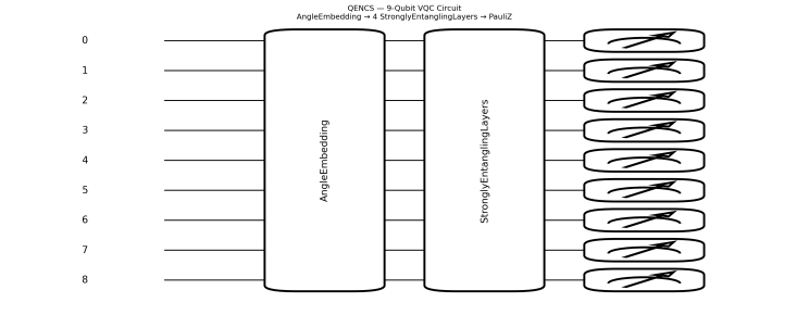
Encoding — AngleEmbedding:
φᵢ = xᵢ · π, where xᵢ ∈ [0, 1]
Each scaled feature becomes a rotation angle applied to a qubit — mapping the band-power value to a point on the Bloch sphere. This is amplitude encoding in the rotation basis: the feature is not stored as a classical value but as the angle of a quantum rotation gate.
Circuit — 4 StronglyEntanglingLayers:
Each layer applies a sequence of parameterised single-qubit rotations (Rot gates — Rz·Ry·Rz decomposition) followed by a CNOT entanglement pattern across the 9-qubit register. With 4 layers, every qubit becomes correlated with every other qubit through the entanglement structure.
Weight tensor shape: (4, 9, 3) — 108 trainable parameters
Each of the 3 parameters per qubit per layer corresponds to the three rotation angles in the Rot gate decomposition.
Measurement:
⟨Z₀⟩, ⟨Z₁⟩, … ⟨Z₈⟩
The expectation value of the PauliZ operator on each qubit — a real number in [-1, 1] representing the probability bias toward |0⟩ vs |1⟩ for that qubit.
Classical output layer:
9 × ⟨PauliZ⟩ → Linear(9, 1) → Sigmoid → lapse probability ∈ [0, 1]
This hybrid quantum-classical architecture delegates feature interaction to the quantum circuit and binary classification to the classical output layer.

Training setup:
Simulator · PennyLane default.qubit (classical CPU simulation) Optimiser · Adam, lr = 0.01 Loss · BCEWithLogitsLoss(pos_weight = 2.0) Epochs · 50 · Batch size · 32 Dataset · 2,000 samples (1,000 per class, stratified subset of 12,811 total) Split · 80/20 train/test
Experiment 1 — Baseline: VQC vs SVM
All numbers from data/training_results.json. Nothing estimated or rounded beyond 4 decimal places.
Metric · VQC (9-qubit, 4-layer) · SVM (RBF, C=1.0)
- Accuracy · 0.5225 · 0.5250
- Precision · 0.5116 · 0.5176
- Recall · 0.9900 · 0.7350
- F1 Score · 0.6746 · 0.6074
- Train time · 113.6s · 0.06s
- Loss curve: 0.9734 → 0.9424 across 50 epochs. A decrease of 0.031. Effectively flat.
Both models perform near random chance on a balanced binary classification task where the baseline is 0.50. The VQC’s higher F1 is not a genuine signal, it is an artefact of recall bias. BCEWithLogitsLoss(pos_weight=2.0) applied double the penalty for missing a lapse, pushing the model toward predicting class 1 for almost every sample. Near-perfect recall (0.9900) paired with low precision (0.5116) is the mathematical fingerprint of a model predicting one class overwhelmingly — not one that has learned a real decision boundary.
No quantum advantage. Not on this dataset. Not yet.

Experiment 2 — Adam vs Quantum Natural Gradient
The natural hypothesis after a flat loss curve: the optimiser is wrong for the geometry.
Adam treats the VQC parameter space as Euclidean — applying gradient updates as if the loss landscape is flat. But quantum circuit parameters live on a non-Euclidean manifold. The correct distance metric between parameter configurations is the quantum Fisher information matrix F(θ), which defines the Bures metric on the space of quantum states.
Quantum Natural Gradient applies the update rule:
θₜ₊₁ = θₜ − η · F(θ)⁻¹ · ∇L(θ)
Rather than following the steepest descent in parameter space, QNG follows the steepest descent in the space of quantum states — respecting the information geometry of the circuit. Theoretically, this should produce faster and more stable convergence on VQCs.
So the optimiser was switched and the experiment rerun on identical data.
Metric · Adam · QNG · Delta
- Accuracy · 0.5225 · 0.5000 · -0.0225
- Precision · 0.5116 · 0.5000 · -0.0116
- Recall · 0.9900 · 1.0000 · +0.0100
- F1 Score · 0.6746 · 0.6667 · -0.0079
- Train time · 113.6s · 5885.2s · 51.8x slower
QNG reproduced the same high-recall bias pattern — predicting lapse for every sample — but required 51.8x more compute to arrive at a marginally worse result. The geometry-aware optimiser made no meaningful convergence difference on this dataset under these conditions.
The optimiser was not the bottleneck.

Experiment 3 — Dataset scale: 2,000 vs 12,811 samples
If the optimiser isn’t limiting convergence, perhaps the dataset is too small for the circuit to find meaningful correlations. The full 12,811-sample dataset was used — 9x more data, same hyperparameters, same circuit.
Metric · 2k Subset · Full Dataset · Delta
- Accuracy · 0.5225 · 0.5033 · -0.0192
- Precision · 0.5116 · 0.4912 · -0.0204
- Recall · 0.9900 · 0.9797 · -0.0103
- F1 Score · 0.6746 · 0.6544 · -0.0202
- Train time · 113.6s · 1017.3s · 9.0x longer
More data produced a slightly worse result at 9x the computational cost. The recall bias persisted at the same magnitude. The circuit did not extract additional signal from the larger dataset at these hyperparameters.
Data volume was not the bottleneck either.
Experiment 4 — The three-way comparison that matters
VQC vs SVM vs 3-layer MLP on identical data, identical splits, identical scaler.
Metric · VQC · SVM · MLP
- Accuracy · 0.5225 · 0.5250 · 0.5150
- Precision · 0.5116 · 0.5176 · 0.5079
- Recall · 0.9900 · 0.7350 · 0.9650
- F1 Score · 0.6746 · 0.6074 · 0.6655
- Train time · 113.6s · 0.06s · 1.1s
A 3-layer classical MLP — input(9) → hidden(18) → output(1) — matched the VQC’s F1 score within 0.009 in 1.1 seconds. The quantum circuit required 113.6 seconds to produce effectively the same result a basic feedforward network produces in the time it takes to make a coffee.
All three models are near random chance. None found a real decision boundary. But the VQC was the most expensive path to that result by a significant margin.
What four experiments actually tells us
Three conclusions that hold across all experimental runs:
The optimiser is not the limiting factor. QNG — the theoretically correct choice for VQC parameter optimisation, produced no meaningful improvement over Adam on this dataset. The loss landscape does not have the geometry that makes information-geometric gradient descent advantageous here.
Data volume is not the limiting factor. Scaling from 2,000 to 12,811 samples at fixed hyperparameters produced slightly worse results. The circuit architecture is not the right shape to exploit additional samples without a different feature encoding strategy.
The limiting factor is the problem-circuit match. A classical MLP with 18 hidden units matched the VQC in F1 at 100x the speed. On a classical CPU simulator, with pre-computed band-power features, on a dataset where classical kernels can approximate the relevant feature interactions a 9-qubit VQC is not earning its computational cost.
The mathematical framework for quantum advantage on certain problem classes is sound. The conditions required to observe it in practice are:
→ A problem where the relevant correlations genuinely require exponential classical resources to approximate
→ A circuit architecture matched to the structure of those correlations
→ Real quantum hardware where entanglement and superposition are physical properties — not operations being simulated on classical bits
→ An optimiser matched to the geometry of the specific loss landscape
None of those conditions were fully met here. That’s not a criticism of the approach, it’s a precise statement of what needs to change.
Your Brain Is Running 5 Electrical Symphonies Right Now. We Built a Quantum Circuit to Listen. was originally published in Towards AI on Medium, where people are continuing the conversation by highlighting and responding to this story.