
Benchmarking eight models across three paradigms revealing why accuracy is a deceptive metric for imbalanced text classification
Table of Contents
- The Dataset & Class Imbalance
- What Spam Looks Like in Words
- Phase 1 : The Eight-Model Benchmark
- How All Eight Models Stack Up
- Where Each Model Actually Fails
- Discrimination Ability Across Thresholds
- The Honest Test Under Imbalance
- Phase 2 : Sentiment Enrichment
- Key Lessons
- What’s Next
Every day, an estimated 3.4 billion phishing emails are sent worldwide. Spam detection is one of the oldest problems in machine learning and one of the most instructive. It sits at the intersection of real-world class imbalance and feature engineering trade-offs, highlighting the question that never gets old: do transformers actually outperform simpler models on practical classification tasks?
This article walks through a complete two-phase pipeline I built to answer exactly that.
Phase 1 benchmarks eight models across three paradigms — classical ML, deep learning, and transformers — on the UCI SMS Spam Collection dataset. Phase 2 takes the best-performing model and pairs it with VADER to enrich the full dataset with sentiment labels, producing a richer, analysis-ready output.
1. The Dataset & Class Imbalance
The UCI SMS Spam Collection contains 5,572 labeled SMS messages. Before touching any model, the first step is understanding what we are actually working with which is shown in the class distribution chart.
The bar chart shows the count of ham versus spam messages with exact values annotated above each bar. The result is stark: 4,825 ham messages versus just 747 spam messages, roughly 87% to 13%. The y-axis stretches far beyond the spam bar, making the gap visually impossible to ignore.
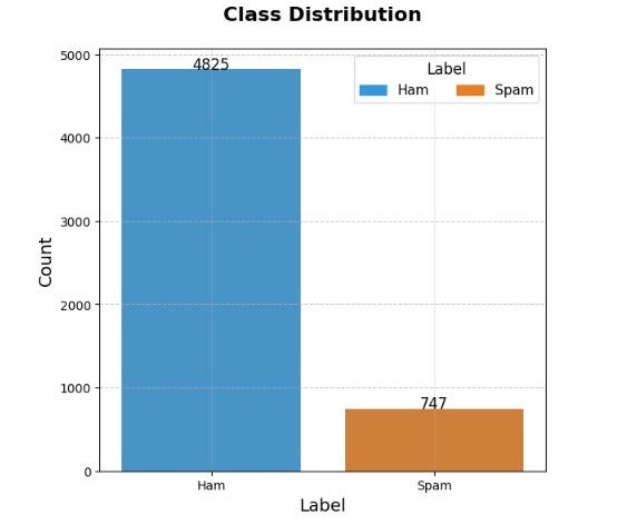
This chart is the entire justification for every metric choice that follows. A model that predicts “ham” for every single message would score 87% accuracy while being completely useless. This is why raw accuracy is disqualified as the primary metric from the outset, and why F1-score, Precision-Recall AUC, and ROC-AUC become the three lenses through which every model is judged.
2. What Spam Looks Like in Words
The side-by-side word clouds are one of the most immediately readable visuals in the project. Each word’s size is proportional to its frequency in that class.

The spam cloud is dominated by words like free, call, now, win, prize, mobile, claim, txt, and urgent. The vocabulary clusters around two psychological levers: urgency (act now, limited time) and reward (win, prize, free). These are the hallmarks of social engineering, crafted to trigger impulsive action before the reader has time to think critically.
The ham cloud looks entirely different. Words like ok, will, come, good, going, time, know, and got dominate the vocabulary of ordinary coordination and conversation. There is no urgency, no reward, no call to action.
This contrast does more than validate the dataset. It reveals why text classification works here: spam and ham are genuinely written in different registers, and that difference is learnable. The word clouds also justify a key preprocessing decision, stopwords are intentionally retained. Words like free, you, now, and call appear frequently in spam and carry genuine signal. A standard stopword list would silently remove some of the most discriminative features in the dataset.
3. Phase 1 : The Eight-Model Benchmark
All models are trained and evaluated on an identical 80/20 train-test split of cleaned text. Every model sees exactly the same 1,115 test messages. This is the non-negotiable foundation of any honest benchmark, if models are tested on different data, the comparison is meaningless.
Three paradigms are represented: classical machine learning (Logistic Regression, SVM, Random Forest, XGBoost) trained on TF-IDF vectors; deep learning (LSTM, BiLSTM) trained on padded integer sequences; and transformers (BERT, GPT-2) fine-tuned on SMOTE-balanced data to counter class imbalance at the batch level.
4. How All Eight Models Stack Up
This grouped bar chart is the headline result of the entire project. Each of the eight models gets four adjacent bars : accuracy (blue), precision (green), recall (red), and F1-score (salmon) , with the exact score annotated above each bar.

A few things stand out immediately.
Accuracy is uniformly high and uniformly misleading. Every model scores somewhere between 0.95 and 0.99. The bars are nearly identical across all eight models. This is the class imbalance effect in action , with 87% of messages being ham, even a mediocre model gets a high accuracy score simply by predicting ham most of the time.
F1-score is where the models actually separate. The spread across models is far more pronounced on F1 than on accuracy, making it the metric that genuinely discriminates between good and poor performers.
Recall is the most revealing metric for spam detection. Low recall means spam is being missed, messages slipping through the filter undetected. The deep learning models (LSTM and BiLSTM) show notably stronger recall than the classical models, reflecting their ability to capture contextual patterns that bag-of-words TF-IDF representations miss.
BiLSTM edges out all other models. Across precision, recall, and F1, the bidirectional LSTM consistently ranks at or near the top. Reading the sequence in both directions gives it access to future context when processing each token, particularly important on short SMS messages where a suspicious word near the end of the message should update the interpretation of everything that came before it.
5. Where Each Model Actually Fails
Eight confusion matrices, one per model, each showing the same four-cell breakdown: true negatives (ham correctly identified), false positives (ham incorrectly flagged as spam), false negatives (spam that slipped through as ham), and true positives (spam correctly caught).

For spam detection, the bottom-left cell (false negatives) is the one that matters most.
- A false negative is spam that reached the inbox.
- A false positive is a legitimate message that ended up in the spam folder.
These two errors carry very different costs in the real world, and the confusion matrices let us read them directly.
The classical ML models split into two groups:
Logistic Regression and XGBoost show a reasonable balance, very few false positives (4 and 3 respectively) and 20 false negatives each.
Random Forest is the exception with FP=0 it never flags legitimate mail as spam, but at the cost of missing 132 spam messages, an 88% miss rate on the spam class that makes it the weakest model in the benchmark by a wide margin.
LSTM and BiLSTM improve on the classical models: LSTM reduces false negatives to 16, and BiLSTM achieves FP=0 with FN=17, 17 total errors and the cleanest result among the deep learning models.
BERT is the standout performer of the entire benchmark; with only 2 false positives and 9 false negatives, it produces just 11 total errors, fewer than any other model, and nearly half the error count of BiLSTM. This is where the investment in contextual embeddings pays off most visibly.
GPT-2, by contrast, does not justify its cost: FN=20 puts it level with the classical models, worse than both LSTM and BiLSTM on recall.
6. Discrimination Ability Across Thresholds
The ROC (Receiver Operating Characteristic) curve plots the true positive rate against the false positive rate at every possible classification threshold. A perfect classifier hugs the top-left corner of the plot. A random classifier follows the diagonal. The area under the curve (AUC) summarises discrimination ability in a single number, with all eight models plotted together on the same axes for direct comparison.
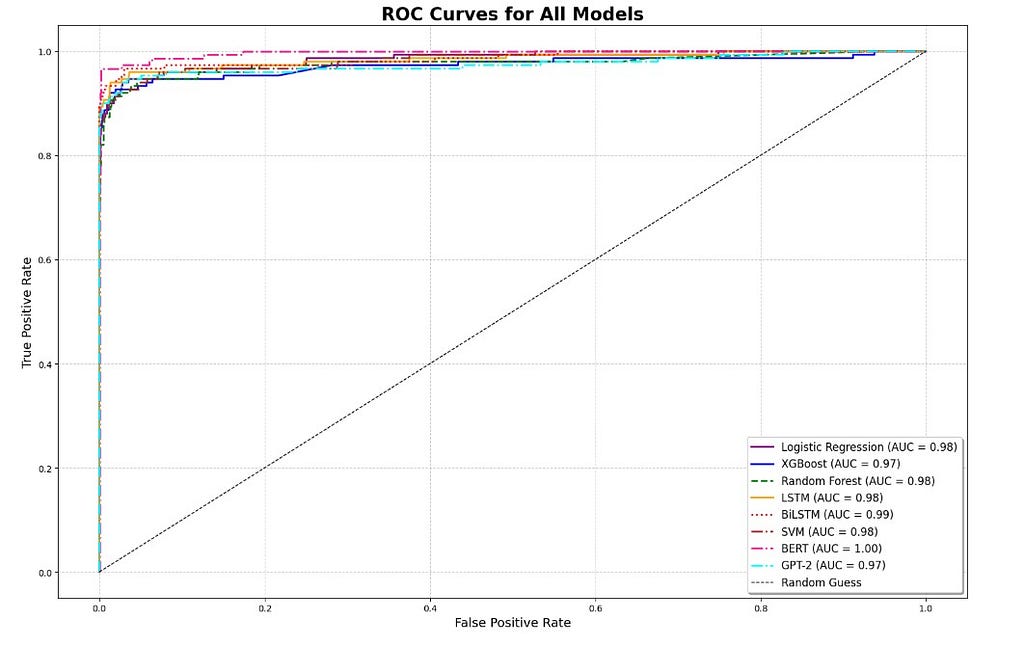
The overall picture is strong across the board. All eight models achieve AUC scores between 0.97 and 1.00, confirming genuine discrimination ability well beyond random chance.
The ROC curve, however, has a known limitation under class imbalance, because the false positive rate is anchored against the large ham population, even modest false positive counts look small as a proportion, making models appear more similar than they are in practice.
The curves are tightly clustered, with most models sitting between 0.97 and 0.99.
BERT is the clear outlier at the top with a perfect AUC of 1.00, followed by BiLSTM at 0.99. Among the classical models, Logistic Regression, Random Forest, and SVM all score 0.98 with XGBoost, at 0.97, is actually the weakest of the four, tying with GPT-2 at the bottom of the ranking.
In the upper-left corner where a spam filter actually operates, high recall at very low false positive rates, BERT and BiLSTM maintain the strongest position, with BERT’s perfect AUC reflecting its ability to separate spam from ham at every threshold.
7. The Honest Test Under Imbalance
The Precision-Recall curve is the most honest evaluation tool for an imbalanced dataset. Unlike the ROC curve, both axes are directly anchored to the minority (spam) class: precision measures what fraction of spam flags were correct, recall measures what fraction of actual spam was caught. The random-classifier baseline is not a flat diagonal but a horizontal line at the spam class prevalence (~13%), making high PR-AUC genuinely difficult to achieve.

The PR curves tell a more nuanced story than the confusion matrices alone.
All models score between 0.95 and 0.99 PR-AUC, confirming strong performance across the board, but the ranking shifts meaningfully from what accuracy or ROC-AUC suggested.
BERT leads at 0.99, followed closely by GPT-2 at 0.98. This is a notable finding: while GPT-2 missed 20 spam messages at the default 0.5 threshold, —matching the weakest classical models — its probability estimates are well-calibrated across all thresholds, placing it second overall on PR-AUC.
This distinction matters: GPT-2 may simply need threshold tuning rather than being written off entirely.
LSTM and BiLSTM both score 0.97, performing identically on this metric and sitting just below the transformers.
The classical models : Logistic Regression and SVM at 0.96, Random Forest and XGBoost at 0.95, occupy the bottom of the ranking, confirming that TF-IDF representations have a ceiling that sequence and contextual models consistently exceed.
All curves remain at high precision until recall reaches approximately 0.85–0.90, after which they drop sharply. This shared drop point reflects a common challenge: the hardest spam messages to catch — borderline cases with ambiguous vocabulary — are difficult for every model regardless of paradigm.
PR-AUC is the final arbiter of this benchmark. It cannot be inflated by the majority class, it directly measures performance on the problem we actually care about, and it captures the full precision-recall trade-off rather than collapsing it to a single threshold.
8. Phase 2 : Sentiment Enrichment
With the classification benchmark complete, the BiLSTM is deployed as an inference engine over all 5,572 messages alongside VADER to produce a sentiment-enriched dataset.
BiLSTM is used here rather than BERT for inference efficiency, at 0.97 PR-AUC it delivers results very close to BERT while running significantly faster over the full dataset. For production use cases where accuracy is the priority, BERT would be the recommended choice.
VADER (Valence Aware Dictionary and sEntiment Reasoner) is a lexicon-based tool that assigns a compound score between -1 and +1 to any piece of text. Above 0.1 is Positive, below -0.1 is Negative, and everything in between is Neutral. It requires no training data, generalises well to informal SMS language, and adds zero labeling overhead, making it the natural choice for enriching a dataset at this scale.
The value of combining both signals is revealed by looking back at the word cloud. Spam vocabulary (free, win, prize, urgent, congratulations) is precisely the vocabulary that VADER scores as strongly positive.
The enriched dataset makes it possible to quantify this hypothesis directly: what fraction of spam messages carry a positive sentiment score, and how does that compare to ham?
The data confirms this: 72.2% of spam messages score Positive, compared to 41.7% of ham, with spam averaging a compound score of 0.445 versus 0.163 for ham. That kind of cross-signal analysis is what transforms the output from a classification exercise into a dataset with genuine downstream research value.
The enriched CSV adds two columns to the original data: vader_score, and sentiment_label.
9. Key Lessons
F1-score, not accuracy, for imbalanced classification:
The class distribution chart makes this visceral. When one class is seven times larger than the other, accuracy is a number that conceals everything important about model performance.
The confusion matrix is where you understand your model’s actual behavior :
Summary metrics tell you how a model scores; confusion matrices tell you how it fails. For spam detection, those are very different questions, and the answers should drive deployment decisions.
PR curves over ROC curves under imbalance :
The ROC curves in this project all look impressive. The PR curves tell a harder, more honest story. When the minority class is 13% of the data, always lead with PR-AUC.
Not all transformers are equal and cost must be weighed against the right model:
BERT is the strongest performer in this benchmark across ROC-AUC (1.00), PR-AUC (0.99), and total errors (11), clearly justifying its training cost.
GPT-2, however, tells the opposite story: despite matching BERT’s parameter scale, it misses 20 spam messages at the default threshold — matching the weakest classical models — while scoring a respectable 0.98 PR-AUC, suggesting its probability calibration is better than its threshold-level recall implies.
The lesson is not that transformers always win or always lose, but that architecture choice matters as much as paradigm. The real strength of a model like GPT-2 is not in its default accuracy but in its reliability across thresholds, its well-calibrated probability estimates allow practitioners to tune the decision boundary to maximise spam recall while keeping the cost of false positives significantly lower than classical alternatives can achieve at the same recall level.
That kind of threshold flexibility is precisely what makes transformer-based classifiers compelling for production spam filters, where the operating point is rarely the default 0.5.
Word clouds are underrated for NLP projects:
Before any model was trained, the spam and ham word clouds already told a complete story about why the task is tractable and which features will matter. Exploratory visualisation belongs at the beginning of the analysis, not as decoration at the end.
10. What’s Next
- Threshold optimisation : shifting the decision boundary below 0.5 to maximise spam recall at a controlled false-positive rate
- Lightweight transformers : benchmarking DistilBERT and TinyBERT, with an explicit runtime comparison against BiLSTM
- More recent corpora : testing generalisation on post-2020 email spam datasets, where phishing language has evolved considerably
- Streamlit dashboard : an interactive interface for real-time spam prediction and sentiment scoring on arbitrary text input
The complete notebook including all eight models, visualisations, and the sentiment enrichment pipeline is available on [Github / Kaggle] .
Thanks for reading! If you found this article useful, feel free to leave a comment or connect. Feedback and questions are always welcome.
From Logistic Regression to GPT-2: Building a Complete Spam Detection & Sentiment Analysis Pipeline was originally published in Towards AI on Medium, where people are continuing the conversation by highlighting and responding to this story.