Chat templates, synthetic data pipelines, deduplication, and the exact failure modes that kill fine-tuned models before training even starts
You spent three days cleaning your data. You wrote the training script. The loss curve looks perfect. You deploy the model, and it generates garbage. You check the loss. Still perfect. You check the eval. Still passing. The model is not broken. The data is broken, and it broke quietly, before training even started.
This article covers every way that happens, and exactly how to prevent it. The focus is the complete lifecycle of fine-tuning data, from the mechanical decisions that must be correct before a single gradient runs, through the strategic choices that determine what capability the model can develop, through the generation, cleaning, and evaluation disciplines that determine whether that capability is real, and through the pipeline-level practices that keep it real across time. Each layer depends on the ones below it. Skipping any layer introduces a failure mode that nothing downstream can fix.
Read the first episode — The Ultimate Transformer Architecture Guide for Fine-Tuners

Table of Contents
- The Non-Negotiable Foundation: Templates, Tokenization, and Loss Masking
- Strategy Before Data: Format Selection and the Quality-over-Quantity Principle
- Manufacturing Training Signal: Synthetic Data, Seed Diversity, and Self-Instruct
- Cleaning, Balancing, and Protecting Signal Integrity
- The Pipeline Level: Reproducibility, Influence Selection, and Collapse Prevention
Chapter 1: The Non-Negotiable Foundation: Templates, Tokenization, and Loss Masking
Before a single gradient update runs, two mechanical decisions determine whether the training signal is coherent or noise, whether the model sees its data in the exact format it was instruction-tuned on, and whether the loss function is computing over the right tokens. Get either wrong and the loss curve will look fine. The model will not be.

1.1 How Model Families Define Structure Through Special Tokens
Every major model family uses a unique schema of special tokens to communicate structure during inference and training. These tokens mark where the user’s message begins, where the assistant’s response begins, where a turn ends, and where the sequence terminates. For Llama 3.x, the markers are <|start_header_id|> tokens wrapping role labels. For Qwen 2.5, the convention is <|im_start|> and <|im_end|>. Mistral uses [INST] and [/INST]. Gemma 2 uses <start_of_turn> and <end_of_turn>.
These are not aesthetic conventions. They are the exact structural markers the model encountered during instruction tuning, and the model’s attention patterns were shaped around them. When fine-tuning data applies a different template, the model reads the role markers as literal text or noise rather than as structural signals. The attention mechanism operates on a corrupted representation. The learned signal degrades, not in a way that triggers an error, but in a way that produces a model that appears to train while internalizing structural noise.
The insidious part, as the Unsloth documentation describes it, is that the loss decreases normally. The training run completes. The model fails at inference. The post-mortem reveals the template was wrong from the first step.
Unsloth handles this through get_chat_template(), which looks up the correct role markers for the specified model family and applies them consistently. The standardize_sharegpt() function handles a related problem: raw datasets often use "human/gpt" role labels rather than "user/assistant," and the chat template application will produce malformed structure if those labels are not normalized first. The processing order matters. Standardize the format, then apply the template.
The practical discipline here is to never construct training data manually against a template written from memory. Use get_chat_template() for the specific model family, verify the output against a known correct sample, and treat any template deviation as a hard error rather than a warning.
1.2 Why Prompt Tokens Contaminate the Gradient
The second mechanical failure mode has a clean mathematical explanation. Standard cross-entropy loss computes over every token in the input sequence. In an instruction-tuning setup, that sequence contains both the user’s prompt and the model’s response. The model is penalized for failing to predict every token, including the tokens of the prompt it was given as input.
The formal loss over a full sequence z = (x, y), where x is the instruction and y is the response, looks like this:
L(z; θ) = -∑(t=1 to |x|+|y|) log P(z_t | z_{<t}; θ)
When restricted to response tokens only, it becomes:
L(z; θ) = -∑(t=|x|+1 to |x|+|y|) log P(y_t | x, y_{<t}; θ)
Every gradient step that includes prompt tokens is computing a partial signal over tokens the model cannot affect at inference time. It is being penalized for not predicting the user’s message, which it will never be asked to generate. The gradient from those positions is noise relative to the actual training objective.
PyTorch’s cross-entropy loss ignores positions labeled with -100. The train_on_responses_only function in Unsloth locates the first response marker in each sequence, scans left to right, and sets all labels preceding that marker to -100. Those tokens remain in the input and continue to contribute to the key-value computation, so context is preserved. They contribute nothing to the loss calculation, so the gradient is clean.
For multi-turn conversations, the same logic extends across turns. Only the assistant’s completions in each turn should generate gradient signal. The user’s messages in subsequent turns are structurally identical to prompt tokens in the single-turn case. Training on them forces the model to predict the human side of a dialogue it will never generate, adding gradient noise at every turn boundary.
The behavioral consequence of skipping this step is measurable. computing loss over the full sequence produces a concrete performance hit relative to response-only training. For tasks requiring precise output structure, the degradation is often visible in early evaluation runs.
Both failures in this chapter share a property that makes them high-priority. Which is, neither produces an obvious error signal. A misaligned template is not a crash. Prompt token contamination is not NaN loss. Both quietly shape the model in the wrong direction from step one, and the farther training proceeds on a corrupted foundation, the harder the damage is to diagnose.
With the mechanical foundation in place, the next two decisions are strategic and must be made before any data is generated, collected, or cleaned. The first is format selection. The second is how to allocate the curation budget.
Chapter 2: Strategy Before Data: Format Selection and the Quality-over-Quantity Principle
2.1 Format as a Capability Decision, Not a Formatting Preference
The format of training data is a structural commitment that determines what the model learns to do and whether it can do it in the deployment context it will actually face.
The Alpaca format stores each example as three discrete fields such as, instruction, input, and output. This structure is well-suited for single-turn tasks where the goal is to perform a specific action given a prompt, such as extraction, classification, or structured generation. The simplicity is a feature for these use cases. The model learns a clean mapping from instruction to completion, and for specialized single-turn models the Alpaca format is a robust and fast bootstrapping choice.
The problem appears when a model trained exclusively on Alpaca data is deployed in a multi-turn chat interface. The ShareGPT and ChatML formats store conversations as ordered lists of message objects, each tagged with a role. This structure is what teaches the model to track context across turns, resolve pronouns against earlier exchanges, and maintain coherence across a conversation arc. A model that has never seen a training signal reinforcing historical continuity will not learn to maintain it. The format choice made at dataset construction time is the capability ceiling at inference time.
The decision must be made at the dataset construction phase, before get_chat_template() is called, because the template interpreter reads role identifiers from the format and constructs the tokenized sequence accordingly. A ShareGPT dataset passed through a template configured for Alpaca, or vice versa, produces structurally corrupted inputs. The Unsloth documentation is explicit about this ordering dependency. Format first, template second, trainer initialization last.
The practical decision is short. If the deployment scenario involves a chat interface or any form of context-dependent interaction, use ShareGPT or ChatML. If the task is single-turn and the deployment scenario is purely task-oriented, Alpaca is sufficient. If the scenario is ambiguous, build for multi-turn. The cost of training multi-turn capable models on single-turn tasks is low. The cost of discovering, after training, that the deployment requires context retention is a full retraining cycle.
2.2 The LIMA Principle: Why Volume Is a Trap for Small Models
In 2023, the LIMA paper produced a result that was genuinely surprising to practitioners who had been treating dataset size as a primary quality lever. A model fine-tuned on 1,000 carefully curated examples matched or exceeded the performance of models trained on 52,000 uncurated samples. The result was not a fluke. AlpaGasus selected approximately 9,000 examples from the original 52,000-sample Alpaca dataset using ChatGPT quality scoring and outperformed the model trained on the full set. The Nuggets study showed that selecting the top 1% of a dataset by quality-first criteria outperformed training on the complete dataset. The DEITA framework optimized jointly for complexity and quality and demonstrated consistent data efficiency gains across model families.
The mechanism behind all of these results is the same. Base models like Llama and Qwen arrive at fine-tuning with factual knowledge and linguistic capability already internalized from pre-training. Fine-tuning does not teach the model what the world is like. It teaches the model the surface form, the output style, the response structure, the reasoning format, the tone. Surface form acquisition requires very little data, provided the examples demonstrating that surface form are consistent and high quality. Noisy, low-quality examples do not just fail to teach the surface form. They actively confuse the model by presenting contradictory signals about what the target behavior looks like.
For small models in the 7B to 8B parameter range, the implication is concrete. The highest return on the data budget comes from cleaning, not accumulation. A well-curated dataset can bring a 7B or 8B model to high performance in under two hours of training. The bottleneck is almost never the volume of data. It is the density of useful signal in the data that exists.
The LIMA principle also clarifies what fine-tuning is not doing. It is not injecting knowledge the base model lacks. If the base model has no representation of a domain, no amount of fine-tuning on task examples will substitute for that missing pre-training coverage. Fine-tuning shapes behavior within the knowledge the model already has. When the target task requires factual knowledge genuinely absent from the base model’s pre-training distribution, that is a signal to reconsider base model selection, not to scale up the fine-tuning dataset.
Format and curation philosophy are now fixed. For most practitioners working in specialized domains, the next problem is immediate and uncomfortable, which is lack of data. Medical documentation is protected. Legal corpora are proprietary. Internal enterprise workflows have never been labeled. The answer the field has converged on is generating synthetic training data from a more capable model, and that answer comes with a failure mode that is easy to miss and expensive to fix.
Chapter 3: Manufacturing Training Signal: Synthetic Data, Seed Diversity, and Self-Instruct

3.1 Teacher-Student Distillation: The Risk Nobody Talks About
Teacher-student distillation works by using a high-capability model, the teacher, to generate instruction-response pairs that a smaller model, the student, is then fine-tuned on. The formal training objective for the student is:
Loss_distill = -∑ log P_student(y_teacher | x)
The existence proofs are real. Vicuna and Koala, both trained on small synthetic datasets derived from proprietary model outputs, demonstrated that distillation from a capable teacher can produce strong open-source models at a fraction of the cost of training from scratch. The approach works. The problem is not the approach. The problem is what practitioners get when they prompt a teacher model without discipline.
Teacher models are verbose. They hedge. They open responses with “That’s a great question…” and close them with “Should i also explain this…” They use markdown headers for three-sentence answers. They over-qualify claims that should be stated directly. A student model trained on this output learns all of it. The distributional mismatch is not between the teacher’s knowledge and the task. The teacher almost certainly knows the domain. The mismatch is between the teacher’s default communication style and the style the deployed student model needs to exhibit.
The mitigation is metaprompting. The teacher’s system prompt must specify the exact output format, response length, tone, and stylistic constraints required at inference time. If the student model is intended to return structured JSON, the teacher must be instructed to return structured JSON in every generated example. If the student should be terse and technical, the teacher must be constrained to terseness and technicality. The quality of the distilled dataset is bounded by the precision of the metaprompt, not by the capability of the teacher. A well-designed metaprompt functions as an automated bridge between the teacher’s default behavior and the student’s target behavior.
One additional constraint applies regardless of metaprompt quality. The diversity of the generated dataset is bounded by the diversity of the seed prompts provided to the teacher. A teacher with unlimited capability but a narrow seed set will generate a narrow dataset. The ceiling on synthetic data quality is the seed, not the model.
3.2 The Self-Instruct Pipeline: Bootstrapping from Minimal Seeds
The Self-Instruct framework, introduced by Wang et al. (2023), addresses the seed diversity problem by using the model’s own generations to expand a small human-written seed set. The original paper bootstrapped from approximately 175 human-written tasks. The pipeline has four stages, and each one has a failure mode worth understanding.
The first stage is instruction generation. The model is prompted with a sample of existing tasks from the pool and asked to generate new ones. The second stage is classification identification, where the model determines whether each generated task is a classification task or an open-ended generation task. This distinction matters for the third stage. Instance generation for open-ended tasks uses an input-first approach, the model generates the input first, then produces the output. For classification tasks, an output-first approach is used, generating the label first and then constructing an input that corresponds to it. This inversion exists specifically to prevent label imbalance. Generating inputs first for classification tasks causes the model to default to majority-class inputs, producing a skewed dataset that will bias the student model toward the same majority class.
The fourth stage is filtering. Generated instructions that are too short, too long, or too similar to existing tasks in the pool are removed. The similarity check uses ROUGE [Recall-Oriented Understudy for Gisting Evaluation] scores. Any generated instruction with a ROUGE-L similarity above a threshold to any existing instruction is discarded. High-quality generations that pass filtering are added back into the task pool, making them available as context for future generation rounds. The pool grows iteratively, and the diversity of later-round generations depends on the quality of earlier-round additions.
The key reframe that Self-Instruct introduces is about where the creative labor lives. The bottleneck in synthetic dataset construction is not generating responses. A capable teacher model can generate thousands of responses per hour. The bottleneck is the seed set. Writing seeds is the work.
3.3 Engineering True Diversity Across Semantic and Syntactic Dimensions
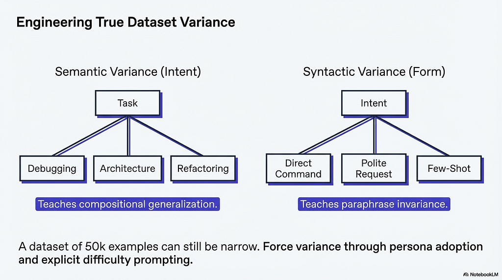
A dataset can contain thousands of non-duplicate examples and still be narrow. If every instruction asks the model to do roughly the same thing in slightly different words, the model learns paraphrase invariance but not compositional generalization. These are different capabilities. Paraphrase invariance means the model handles surface variation of familiar tasks. Compositional generalization means the model handles novel combinations of familiar concepts. The second is what practitioners need from a fine-tuned model, and it requires deliberate diversity engineering at the dataset level.
Research on Flan-T5 and the original Alpaca model demonstrated that models trained on diverse instructions show significantly higher zero-shot generalization than models trained on narrow instruction sets, even when the narrow set contains more total examples. Diversity operates across two distinct dimensions, and conflating them produces an incomplete dataset.
Semantic variance is diversity at the level of intent. For a medical assistant dataset, this means including examples across symptom assessment, diagnosis support, treatment explanation, medication guidance, preventive care, and patient education, spanning multiple conditions, age groups, and varying levels of patient health literacy. If the dataset covers only one or two of these intents at depth, the model will handle those intents well and degrade on the others.
Syntactic variance is diversity at the level of linguistic form. The same underlying task can be expressed as a direct command, a polite request, a few-shot prompt with examples, or an indirect description of the problem without explicitly naming the task. Models trained on only one syntactic form will perform inconsistently when users approach the same task differently.
The practical mechanism for generating both types of variance in synthetic data is explicit teacher prompting. Instructing the teacher to adopt different user personas or vary the difficulty level of the following task produces measurably more diverse outputs than generating without those constraints. The instruction to vary difficulty is particularly useful because it naturally produces examples across the full spectrum from trivial to boundary-pushing, and boundary-pushing examples are where the student model learns the most.
The structural point connecting all three subsections in this chapter is that synthetic data quality is a function of upstream decisions. The teacher’s capability sets an upper bound. The metaprompt determines how much of that capability transfers into usable format. The seed set determines the coverage of the generated distribution. Deliberate variance engineering determines whether that distribution is wide enough for the model to generalize.
The data now exists. The format is correct. The generation pipeline produced thousands of examples with reasonable coverage and controlled style. This is the moment most practitioners treat as done and initialize the trainer.
Chapter 4: Cleaning, Balancing, and Protecting Signal Integrity
4.1 Deduplication: Exact, Near, and Semantic
Duplicates in a fine-tuning dataset are more damaging than duplicates in a pre-training corpus. Pre-training operates at a scale where a few repeated examples are statistically negligible. Fine-tuning operates on hundreds to tens of thousands of examples, where repeated examples represent a meaningful fraction of the gradient signal. A model that sees the same example or near-identical variants multiple times does not generalize from that example. It memorizes it. The downstream symptom is a model that collapses into repetitive generation for inputs resembling the duplicated examples while performing inconsistently on everything else.
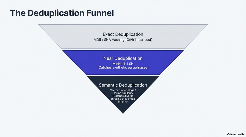
Exact deduplication is the cheapest fix in all of machine learning. MD5 or SHA hashing produces a fingerprint for each example, and any fingerprint appearing more than once identifies a duplicate. The computational cost is linear in dataset size.
Near-duplicate detection is harder and more important for synthetic datasets specifically. A generation pipeline that produces multiple batches from overlapping seeds will create paraphrases, examples that are not character-identical but are close enough in structure that the model treats them as the same signal. MinHash LSH [Locality-Sensitive Hashing] handles this by decomposing each text into character n-grams called shingles, computing a compact signature through multiple hash functions applied as random permutations, and using a banding technique to group signatures with high Jaccard similarity into the same buckets. Two texts landing in the same bucket are flagged as near-duplicates. The elegance of this approach is that it avoids pairwise comparison entirely. Pairwise comparison over a dataset of 50,000 examples requires over a billion comparisons. MinHash LSH achieves near-duplicate detection in sublinear time relative to dataset size.
Semantic deduplication goes one level further by using vector embeddings to identify examples that express the same intent with different surface forms. Two instructions that ask the model to summarize a legal document, one phrased as a command and one phrased as a polite request with completely different vocabulary, will pass both hash-based and MinHash checks but carry the same learning signal. Semantic deduplication via embedding similarity catches these. The computational cost scales quadratically for naive pairwise comparison, though approximate nearest neighbor indices bring it to manageable levels for typical fine-tuning dataset sizes.
4.2 Class Balance and Decision Boundary Engineering

For classification, detection, and refusal tasks, the distribution of labels in the training set is the primary determinant of the model’s decision boundary. The failure mode from class imbalance is not subtle. A safety detection model trained on data where 99% of examples are labeled safe will learn, correctly by the loss function’s logic, that predicting safe for every input minimizes training loss. The model achieves high accuracy and zero practical utility.
Four techniques address class imbalance, each at a different level of the training pipeline. Random oversampling duplicates minority class examples to increase their gradient frequency, with the risk of overfitting to specific phrasings within the minority class. Random undersampling removes majority class examples to prevent them from dominating the loss, with the risk of discarding genuine distributional information. Weighted loss functions, configurable in SFTTrainer, assign higher loss values to minority class predictions without modifying the dataset itself. Focal loss dynamically downweights the loss contribution from easy examples regardless of class, concentrating gradient signal on the hard examples where the decision boundary is actually uncertain.
Hard negatives are the most valuable and most difficult component of a well-balanced dataset for detection tasks. A hard negative is an example that superficially resembles the positive class but should be classified negatively. In a toxic speech detector, a hard negative might be a sentence containing a sensitive term used in a clinical context, an academic citation, or ironic commentary. A model that has never seen hard negatives during training only learns the positive class boundary. It will activate on inputs that contain surface features of the positive class without understanding the contextual features that distinguish genuine positives. The result is high false positive rates on exactly the kinds of inputs that appear in real usage.
Generating hard negatives synthetically requires explicit teacher prompting. The effective pattern is instructing the teacher to generate examples that look like category X but should be classified as category Y, with specific constraints on what makes the example boundary-case rather than obviously negative. Weak negatives, examples clearly unrelated to the positive class, are easy to generate and provide weak learning signal. Ambiguous examples, where the correct classification is genuinely unclear, teach the model to request clarification rather than commit to a low-confidence prediction. A complete dataset for a detection task contains all four example types, positive, weak negative, hard negative, and ambiguous, in proportions that reflect the actual distribution the model will encounter in production.
4.3 Evaluation Integrity and Pre-Training Contamination
The most consequential data hygiene decision in the entire pipeline must be made before generation begins. Which is constructing the evaluation set first, from real-world or manually curated data, before any synthetic training examples are generated.
The failure mode from violating this order is eval set contamination. When training data and evaluation data are generated by the same pipeline from the same seed prompts, the teacher model will produce training examples that are semantically identical to evaluation reference answers. The model’s performance on the contaminated eval set looks strong. Its performance on actual user inputs looks weak.
Distribution shift, where production inputs differ systematically from training data, is according to multiple LLM deployment guides the primary failure mode for deployed models. Deduplication prevents the model from over-indexing on specific phrasings. Class balance ensures the decision boundary reflects the true task structure. Evaluation integrity ensures that the metrics guiding development decisions are measuring the right thing. A model that passes all three checks before training has a substantially higher probability of performing on the inputs it will actually receive.
The dataset is now clean, balanced, and evaluated against a meaningful benchmark. The remaining questions are about the pipeline itself, whether it can be reproduced, whether the most influential examples can be identified before training rather than after, and whether the pipeline will remain stable across multiple iterations or collapse into a narrowing loop of self-generated noise.
Chapter 5: The Pipeline Level: Reproducibility, Influence Selection, and Collapse Prevention
5.1 Reproducibility as Engineering Discipline
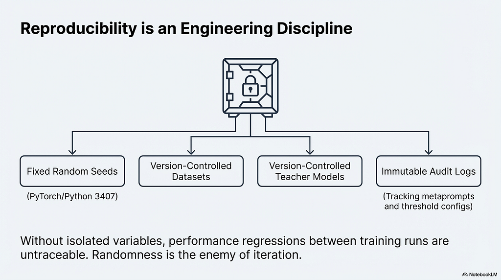
The diagnostic value of any fine-tuning run depends entirely on the ability to isolate variables. If the generation process contains uncontrolled randomness, whether from temperature sampling without a fixed seed, dataset shuffling without a fixed order, or teacher model version drift between runs, then a performance regression between two training runs cannot be attributed to any specific cause. The model changed, or the data changed, or both changed, and there is no way to know which.
The minimum reproducibility requirements for a fine-tuning pipeline are fixed random seeds for both PyTorch and Python’s random module, explicit versioning of the dataset used for each training run, explicit versioning of the teacher model used for generation, and audit logs recording the exact prompt templates and filtering thresholds applied to each generation batch.
The practical consequence of skipping this discipline is what engineers sometimes call chasing ghosts. A model trained on Monday outperforms the model trained on Friday. The Friday run used a slightly different generation temperature, a teacher model that received a silent update, and a shuffle order that placed all hard examples in the final training steps where they received fewer gradient updates due to learning rate decay. None of these changes were logged. The team spends a week investigating the model architecture before discovering the data was different. Reproducibility is not overhead. It is the foundation that makes iteration possible.
5.2 Influence-Based Selection: LESS and the 5% Principle
The LIMA principle from Chapter 2 established that a small, high-quality dataset outperforms a large, uncurated one. LESS [Low-rank gradiEnt Similarity Search], introduced by Xia et al. (2024), makes that principle operational by providing a mechanism for identifying which specific examples are high-quality relative to a target task, before training on them.
The mechanism is gradient-based. LESS scores each candidate training example by computing the similarity between its gradient and the gradients of a small validation set representing the target capability. Examples whose gradients align strongly with the validation set gradients will, when trained on, push the model in the direction that improves performance on the target task. Examples whose gradients are misaligned push the model in irrelevant or counterproductive directions, consuming gradient budget without contributing to the target capability.
Training on a LESS-selected 5% of the data can often outperform training on the full dataset across diverse downstream tasks. This means that for many fine-tuning scenarios, the vast majority of examples in a dataset contribute neutral or counterproductive gradient signal relative to the target task, and the influential minority can be identified before training begins.
For practitioners who cannot implement full LESS gradient scoring, the principle informs manual curation decisions. The examples that sit near the decision boundary of the target task, the ones that require the model to handle genuine ambiguity, apply nuanced reasoning, or resolve competing constraints, are the examples that drive the most learning. Easy examples, where the correct response is obvious and consistent with the base model’s existing behavior, contribute minimal gradient signal. Prioritizing hard, informative examples over easy, redundant ones is the manual approximation of what LESS automates.
5.3 Multi-Turn Construction and Intent Trajectories
Single-turn fine-tuning teaches the model to respond to isolated prompts. It does not teach the model to maintain coherence across a conversation, resolve pronouns against prior turns, or progressively extract information from a user toward a goal. These are learned behaviors, and they require training data that demonstrates them.
The ShareGPT format from Chapter 2 is the structural prerequisite. The quality of multi-turn data depends on something beyond format and conversations must have intent trajectories. An intent trajectory is a global structure that orients the conversation toward a goal across multiple turns, rather than treating each turn as an independent exchange. Without intent trajectories, generated multi-turn data drifts. The model learns to produce locally coherent responses but fails to move conversations forward productively. Research on the ConsistentChat framework, published at EMNLP 2025, showed that models trained on skeleton-guided multi-turn dialogues designed with explicit intent trajectories achieved 20 to 30% better chat consistency than models trained on existing single-turn and multi-turn instruction datasets.
5.4 Model Collapse in Iterative Pipelines
The most dangerous failure mode in modern fine-tuning pipelines unfolds slowly across multiple training iterations. As the field moves toward pipelines where a fine-tuned model generates synthetic data for the next training cycle, each generation of data can become slightly less diverse than the previous one. In such scenario, the model generates from its own learned distribution. That distribution is already narrower than the human data it was trained on. The next generation narrows further. Over successive iterations, the model converges toward a mode, generating high-confidence outputs that represent the center of its learned distribution while losing the rare events, edge cases, and nuanced examples that made earlier generations valuable.
The research on model collapse formalizes this risk as:
Risk_collapse ∝ Iterations × (Synthetic Data Ratio / Real Data Anchor)
The ratio that matters is synthetic data relative to real data at each iteration. A pipeline that introduces no new real-world data across iterations will collapse. The rate of collapse scales with the number of iterations and the proportion of synthetic data in each cycle. A pipeline that anchors each iteration with fresh human-generated or real-world seed examples maintains diversity by continuously injecting signal from outside the model’s current distribution.
The practical implication is that iterative synthetic pipelines require a deliberate anchoring strategy. Each generation cycle should introduce new real-world seed prompts, human-reviewed examples, or expert-curated edge cases that the current model cannot have memorized. Without this injection, the model does not improve across iterations. It decays into a narrow, repetitive, and confidently wrong version of itself.
Conclusion
This is where the data-centric view of fine-tuning arrives at its full conclusion. Mechanical alignment from Chapter 1 ensures the signal reaches the model correctly. Format and curation philosophy from Chapter 2 ensure the signal is worth sending. Synthetic generation from Chapter 3 ensures the signal covers the right distribution. Cleaning, balancing, and evaluation integrity from Chapter 4 ensure the signal is not corrupted before training begins. Pipeline discipline from Chapter 5 ensures the signal remains valid and improvable across the lifetime of the system.
Each layer depends on the ones below it. Skipping any layer introduces a failure mode that the remaining layers cannot compensate for. The data is not a prerequisite to the real work. The data is the work.
Connect with me on LinkedIn: https://www.linkedin.com/in/suchitra-idumina/
Note — The primary purpose of the images (slides) is to provide intuition. As a result, some oversimplifications or minor inaccuracies may be present.
The Ultimate Fine-Tuning Data Guide for Engineers: How to Fine-Tune Correctly, Part 3 was originally published in Towards AI on Medium, where people are continuing the conversation by highlighting and responding to this story.