How I built a molecular similarity search system using ChemBERTa, RDKit, and a vector database, and what I learned along the way.
Why I Wanted to Do This
I have been spending a lot of time lately experimenting with vector databases and embedding-based search.
Most examples I came across focused on text: semantic document search, FAQ retrieval systems, or chatbot memory.
At some point, I started thinking: could the same idea work for molecules?
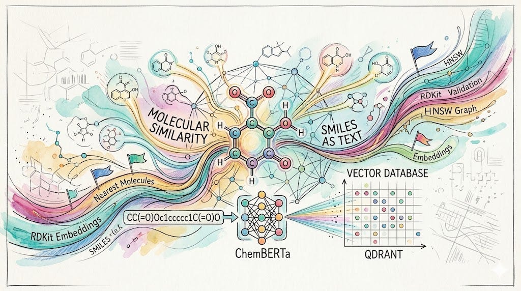
Around that time, I had also been reading about ChemBERTa, a transformer model trained on SMILES strings from the ZINC database. What caught my attention was that molecules could be written as plain text using something called SMILES (Simplified Molecular Input Line Entry System). For example, aspirin can be written as a simple string like CC(=O)Oc1ccccc1C(=O)O.
Seeing a molecule represented as text immediately made me wonder whether the same transformer models used for language might be able to learn patterns in molecular structures too.
The idea that you could feed those SMILES strings into a transformer and get a meaningful vector representation out of them was genuinely intriguing to me. Around the same time, Qdrant had released a clean Python client with native support for payload filtering.
That made me wonder what would happen if these two things actually worked together.
So I decided to build a small experiment and find out. It took multiple attempts and more than a few long nights of debugging to get the pipeline working end-to-end, but the process itself turned out to be surprisingly fun.
A quick note before we go further: you do not need a PhD in chemistry to follow along. A little familiarity with molecules helps, but I have tried to keep the explanations simple and focus on the system and the ideas behind it.
Here is what the system ended up doing:
- Download and cache the ZINC-250k dataset (a collection of drug-like molecules from the ZINC database)
- Validate and canonicalize (converting data with multiple possible representations into a single form) each SMILES string using RDKit, converting it into a single standard representation and computing a heuristic toxicity score
- Generate 768-dimensional molecular embeddings using ChemBERTa
- Store those embeddings in Qdrant together with molecular property metadata
- Query the index using cosine similarity with optional filters such as molecular weight and LogP (a measure of fat vs. water solubility)
- Serve the results through either a FastAPI endpoint or a Streamlit interface
This article demonstrates how the whole system came together step by step.
If you are a developer or someone curious about vector search or transformer embeddings and want to see what happens when you apply those ideas outside of text, this is a good place to start.
The Problem I Wanted to Test

When I started reading about molecule search pipelines, I noticed that most of them rely on something called fingerprint similarity.
The basic idea is fairly straightforward. You take a molecule and convert it into a compact numerical representation called a Morgan fingerprint. You can think of it as a long list of 0s and 1s that records which fragments or substructures appear in the molecule.
Once every molecule has this representation, comparing two molecules becomes simple. You measure how much their fingerprints overlap. That overlap is measured using a Tanimoto score, a standard similarity metric in cheminformatics. The score ranges from 0 to 1, where 0 means the molecules share no fragments at all, and 1 means their fingerprints are identical.
For obvious structural matches, this works very well. It is fast, simple, and easy to reason about.
But while I was testing it on a small set of compounds, I kept noticing something odd. Sometimes two molecules looked chemically related when I inspected them manually, but the system failed to surface them. They shared some structural character, yet the fingerprint overlap was too small for the Tanimoto score to reflect that relationship.
That gap is what pushed me to try something different.
The underlying issue is that fingerprints compress a molecule into that list of 0s and 1s. During that compression, different substructures can end up mapped to the same position in the vector. When that happens, the fingerprint loses information before you even run the query. In practice, you are no longer searching for the molecule itself, but a simplified representation of it.
This becomes especially obvious in something chemists call scaffold hopping. That is when two molecules act on the same biological target but have completely different structural cores. In those cases their fingerprints can look very different, even though they may be functionally related. Since the Tanimoto score only measures fragment overlap, it has no way of catching that relationship.
There is also something known as an activity cliff. Sometimes a very small structural change can dramatically alter how a molecule behaves biologically.
For example, adding a single methyl group, which is just one carbon atom with three hydrogens, can significantly change a molecule’s activity. But in a fingerprint representation that modification might appear as just a one-bit difference, without capturing the chemical importance of the change.
Then there is the scaling problem.
Tanimoto similarity is essentially a linear scan. Every query molecule has to be compared with every molecule in the dataset, one by one. When you start dealing with millions of compounds and thousands of queries, that quickly turns into billions of comparisons. At that point, you need additional engineering just to keep the system running efficiently.
None of these issues was a deal breaker for the small experiment I had in mind. But they were enough to make me curious whether a different approach, one that learns patterns in molecular structure instead of just counting fragments, might do a better job.
The Idea

Most molecule search systems represent molecules using fingerprint vectors. In practice, that means breaking a molecule into fragments, hashing those fragments into a fixed-length bit vector, and then comparing molecules using a similarity score like Tanimoto.
This approach works well when two molecules share obvious structural fragments.
But while exploring these systems, I kept wondering whether there was another way to represent molecules that captured more than just fragment overlap.
Instead of encoding molecules as fragment bits, I wanted to try converting each molecule into a dense vector that represents its overall structure. The intuition was simple: if two molecules are structurally similar, their vectors should end up close to each other in that space, even if they do not share the exact same fragments.
That is where ChemBERTa comes in.
ChemBERTa is a transformer model trained on SMILES strings from the ZINC database. A SMILES string is simply a way of writing a molecule as text. Because molecules can be represented as text strings, a transformer can learn patterns in those strings in much the same way language models learn patterns in sentences.
During training, the model hides parts of a SMILES string and tries to predict the missing pieces. By repeating this process across millions of molecules, it gradually learns common structural patterns.
When you pass a SMILES string through the model, it produces a vector of 768 numbers. You can think of this vector as the model’s internal representation of that molecule. Molecules that are structurally similar tend to produce vectors that end up close to each other in this space.
One thing worth being clear about is what these vectors actually represent. They capture structural similarity, meaning the model learns patterns in how molecules are built. They do not directly tell you how molecules behave biologically. ChemBERTa was trained only on molecular structures, not on experimental data such as binding assays or toxicity measurements. So what the model learns is structural patterns, not biological activity.
Once molecules are represented as vectors, searching becomes much easier.
Instead of comparing a query molecule against every molecule in the dataset one by one, you can simply search for the nearest vectors in that space. That is where a vector database becomes useful.
In this project, Qdrant handles that part. It indexes the vectors and retrieves the ones closest to the query very quickly. I experimented with a few different vector databases before settling on Qdrant, which I will explain in the next section.
How the Pipeline Fits Together
Once I had the pieces figured out, the overall pipeline ended up being surprisingly simple.
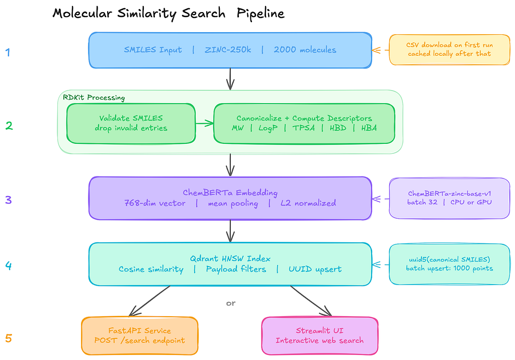
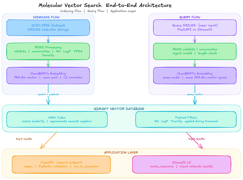
The system is basically five stages, where each step does one clear job before passing the data to the next one:
SMILES strings
 │
 ▼
RDKit validation and canonicalization
 │
 ▼
ChemBERTa embedding (Hugging Face Transformers)
 │
 ▼
Qdrant vector indexing (upsert with metadata payloads)
 │
 ▼
Similarity search API (FastAPI) or Web UI (Streamlit)
The process starts with raw SMILES strings.
These are just text representations of molecules. Before doing anything else, I run them through RDKit to validate and standardize them.
If a string does not parse into a valid molecule, it gets discarded immediately. Even in curated datasets, there are always a few entries that fail validation, so catching them early avoids problems later in the pipeline.
Once the molecules are validated, the canonical SMILES strings go into ChemBERTa (seyonec/ChemBERTa-zinc-base-v1 from Hugging Face). The model processes each SMILES string and produces a vector representation. Since the model outputs token-level embeddings, I apply mean pooling on the final hidden layer to produce a single 768-dimensional vector for each molecule.
These vectors are then stored in Qdrant along with useful metadata such as molecular weight and LogP, which measures how soluble a molecule is in fat versus water. Each molecule becomes a point in the vector collection, with the embedding as the vector and the descriptors stored as payload metadata.
Under the hood, Qdrant builds an HNSW index over these vectors.
HNSW (Hierarchical Navigable Small World) is a graph-based data structure designed for fast approximate nearest neighbour search. Instead of scanning every vector in the dataset, it navigates the graph to quickly find candidates that are closest to the query vector.
- At query time, the same ChemBERTa model converts the input molecule into a vector.
- Qdrant then performs a k-nearest neighbour search using cosine similarity to find the closest molecules in the index.
Because the molecular properties are stored as payload metadata, filters like molecular weight or LogP can be applied directly during the search instead of filtering results afterwards.
The final layer of the system is just an interface: either a FastAPI endpoint for programmatic access or a Streamlit UI for exploring results interactively.
Why I Chose Qdrant
The core requirement I had was simple: I needed a vector search that could apply numeric filters on molecular properties during retrieval, not after it. That one requirement ruled out more options than I expected.
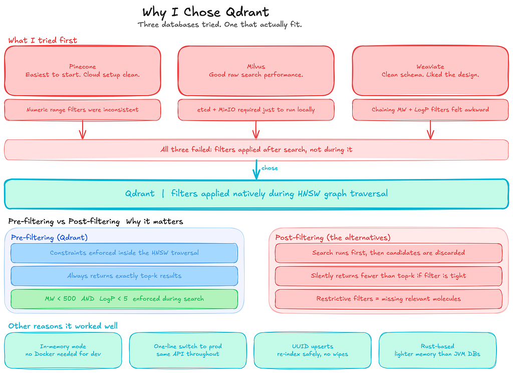
Before settling on Qdrant, I tried three different vector databases.
- Pinecone was the easiest to get running. Cloud setup was straightforward, and the basic vector search worked fine. The problem showed up when I tried to combine similarity search with numeric range filters on molecular weight and LogP. The filtering behaviour was inconsistent and harder to reason about than I wanted.
- Milvus gave good raw vector search performance, but the local installation required spinning up etcd and MinIO just to run a development experiment. That overhead was not acceptable for something I was iterating on quickly.
- Weaviate had a clean schema system that I liked, but chaining multiple numeric range filters together with a vector search query felt awkward. The semantics were not intuitive enough for the kind of queries this use case needed.
Qdrant solved the specific problems the others did not.
The thing that mattered most was how it handles filters. In this kind of search, you rarely query by vector alone.
You want to say: find molecules similar to this one, but only where the molecular weight is under 500, and LogP is below 5.
Qdrant applies those constraints natively during the HNSW graph traversal, not after. Post-filtering sounds like the same thing, but it is not. If your filter is restrictive, you silently end up with fewer than top-k results because candidates are removed after the search has already finished.
That was not acceptable for how I wanted the search to behave.
The in-memory client (QdrantClient(“:memory:”)) was also a big advantage during development. Qdrant can run in a few different ways. You can connect to a standalone Qdrant server running in Docker, you can run it as a persistent service storing data on disk, or you can use the lightweight in-memory mode provided by the Python client.
For this experiment, the in-memory option made the most sense. It let me run the entire pipeline directly on my laptop without starting Docker or managing an external service. The collection exists only for the lifetime of the process, which is perfectly fine when you are iterating quickly and rebuilding the index repeatedly while debugging the pipeline.
Once the pipeline worked end-to-end, switching to a persistent Qdrant deployment was straightforward. The only change required was replacing the in-memory client with a connection to a running Qdrant server. Because the API stays the same, the rest of the code did not need to change. That made the development loop fast while still keeping the path to production simple.
Beyond those two things, the indexing behaviour was predictable. Non-destructive collection creation, deterministic UUID-based upserts from canonical SMILES, and explicit payload index creation. None of it required workarounds.
The HNSW parameters (m, ef_construct, ef at query time) are directly tunable. And the Rust-based memory footprint is noticeably lighter than the JVM-based alternatives when you are running 768-dimensional embeddings on consumer hardware.
When to Use Embeddings vs. Fingerprints

This question came up a lot while I was building this system, so I would like to talk about it.
If you are working with a group of molecules where the relationships between structure and activity are already well understood, traditional fingerprint similarity is usually the better choice.
Methods like ECFP4 (Extended Connectivity Fingerprints, a commonly used Morgan fingerprint variant) combined with the Tanimoto similarity score are simple, fast, and easy to interpret.
These approaches represent each molecule as a fixed-length bit vector that records which structural fragments are present. When two molecules share many of the same fragments, the Tanimoto score between them will be high. In situations where molecules share obvious structural patterns, this approach works extremely well and has been the standard technique for years.
In those cases, introducing a transformer model and a vector database only adds complexity without providing much practical benefit.
Embeddings start to become useful in a different kind of situation.
Sometimes, two molecules can behave similarly even though they do not share obvious fragments in their structure.
Fingerprint methods struggle in these cases because they only capture explicit substructures that appear in the molecule. Embedding models like ChemBERTa work differently. Instead of recording fragments directly, they learn broader structural patterns from large datasets of molecules.
The model converts each molecule into a dense vector representation, and molecules that share similar structural or physicochemical characteristics tend to end up close together in that vector space. Because of this, embedding-based search can sometimes surface candidate molecules that fingerprint similarity would completely miss.
ChemBERTa is the model I used for this experiment, but it is not the only possible choice. Mol2Vec generates smaller embeddings and runs faster on CPUs, which can make it attractive for large-scale pipelines. Graph neural network (GNN) models can go even further by learning representations directly from molecular graphs and incorporating three-dimensional structural information, which can matter when molecular shape influences how a compound binds to a biological target. I chose ChemBERTa mainly because it works directly with SMILES strings and is well supported in the Hugging Face ecosystem, which made it easy to integrate into the pipeline.
Similarity Metric
Before indexing, every embedding vector is L2 normalized. In simple terms, this means each vector is scaled so its length becomes 1. After normalization, the vectors all lie on the surface of a unit sphere. The direction of the vector still represents the molecule, but differences in magnitude are removed.
The reason for doing this is practical:
Once vectors are normalized, cosine similarity and dot product produce the same ranking of results. In other words, comparing vectors by their angle (cosine similarity) becomes equivalent to using a dot product because all vectors have the same length.
I chose cosine similarity mainly because the scores are easier to interpret when looking at search results.
- Cosine scores fall between -1 and 1, so seeing values like 0.92 or 0.68 gives you an immediate sense of how similar two molecules are.
- That makes debugging retrieval behaviour much easier when you are trying to understand why certain molecules appear in the results.
Without normalization, dot product similarity is another common option. However, dot product scores can vary widely depending on vector magnitude, which makes them harder to interpret directly. Two vectors might have a high score simply because they are large, not necessarily because they point in the same direction.
Other similarity metrics are possible as well.
Euclidean distance is sometimes used in vector search systems, especially when magnitude differences carry useful information.
In this case, though, the direction of the embedding matters more than its length, so cosine similarity with normalized vectors end up being the simplest and most stable choice and it also gives the best results.
Environment Setup
Everything runs on Python 3.10+, and all dependencies come straight from PyPI. No custom forks, no proprietary packages.
# Core cheminformatics
pip install rdkit

# Transformer framework, tokenizer, and PyTorch
pip install transformers torch

# Vector database client (requires Qdrant server v1.10+ for the Query API)
pip install "qdrant-client>=1.10.0"

# Web interface dependencies (select appropriate stack)
pip install fastapi uvicorn
# or
pip install streamlit
A couple of things to know before you start:
The PyPI package is just called rdkit. It used to be published as rdkit-pypi, so if you see older references to that name, they mean the same thing. The codebase uses the X | Y union type syntax (e.g., dict | None), which requires Python 3.10 or above, so make sure you are not on an older version. And for the model itself: ChemBERTa runs fine on CPU for smaller datasets, but if you are planning to process anything over 100k molecules, GPU inference is going to save you a lot of time.
Building It: Step by Step
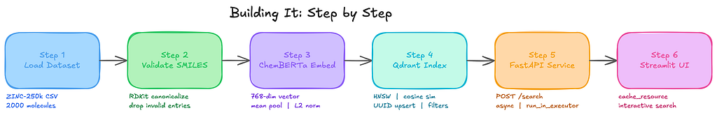
Step 1: Load the Dataset and Validate SMILES
The first thing I realized while building this is that SMILES strings from real databases are messy.
The same molecule can be represented in multiple valid ways. Some entries contain salts or stereoisomer annotations. Others are just flat-out invalid. Feeding any of that directly to a transformer model would produce either garbage embeddings or silent failures.
For the dataset, I went with ZINC-250k, a widely used benchmark subset of drug-like molecules from the ZINC database. This is the same source ChemBERTa was pre-trained on, which makes it a natural fit. The data loader downloads the CSV on first run, caches it locally, and returns validated, deduplicated SMILES:
from __future__ import annotations

import csv
import logging
from pathlib import Path
import urllib.request

from rdkit import Chem
from molsearch.config import DATA_CACHE_DIR, DATASET_SIZE


logger = logging.getLogger(__name__)

ZINC_250K_URL = "https://raw.githubusercontent.com/aspuru-guzik-group/chemical_vae/master/models/zinc_properties/250k_rndm_zinc_drugs_clean_3.csv"
ZINC_FILENAME = "zinc_250k.csv"


# Fallback molecules if the download fails (for offline/CI environments)
_FALLBACK_SMILES: list[str] = [
    "CC(=O)Oc1ccccc1C(=O)O",  # Aspirin
    "CC(C)Cc1ccc(cc1)C(C)C(=O)O",  # Ibuprofen
    "CC(=O)Nc1ccc(O)cc1",  # Acetaminophen
    "O=C(O)Cc1ccccc1Nc1c(Cl)cccc1Cl",  # Diclofenac
    "COc1ccc2cc(CC(C)C(=O)O)ccc2c1",  # Naproxen
]


def load_dataset(
    max_molecules: int = DATASET_SIZE,
) -> tuple[list[str], list[float | None]]:
    """
    Load molecules from the ZINC-250k dataset.
    Downloads on first call and caches locally for subsequent runs.
    Returns validated, deduplicated SMILES. Toxicity scores are None
    because ZINC has no toxicity annotations - they get computed
    dynamically in molecule_processor.py.
    Falls back to a small built-in list if the download fails.
    """

    cache_dir = Path(DATA_CACHE_DIR)
    cache_dir.mkdir(parents=True, exist_ok=True)
    cache_path = cache_dir / ZINC_FILENAME

    if not cache_path.exists():
        try:
            logger.info("Downloading ZINC-250k from %s …", ZINC_250K_URL)
            urllib.request.urlretrieve(ZINC_250K_URL, str(cache_path))
        except Exception:
            logger.warning(
                "Download failed; using %d fallback molecules",
                len(_FALLBACK_SMILES),
            )
            smiles = _FALLBACK_SMILES[:max_molecules]
            return smiles, [None] * len(smiles)

    seen: set[str] = set()
    valid_smiles: list[str] = []

    with open(cache_path, newline="", encoding="utf-8") as f:
        reader = csv.DictReader(f)

        for row in reader:
            raw = row.get("smiles", "").strip()

            if not raw:
                continue

            mol = Chem.MolFromSmiles(raw)
            if mol is None or mol.GetNumAtoms() == 0:
                continue

            canonical = Chem.MolToSmiles(mol)

            if canonical in seen:
                continue

            seen.add(canonical)
            valid_smiles.append(canonical)

            if len(valid_smiles) >= max_molecules:
                break

    toxicity_scores: list[float | None] = [None] * len(valid_smiles)

    logger.info("Dataset ready: %d molecules", len(valid_smiles))

    return valid_smiles, toxicity_scores
By default, DATASET_SIZE is 2000 molecules, controlled via the MOLSEARCH_DATASET_SIZE environment variable. The toxicity scores returned here are all None.
That is intentional as ZINC does not include toxicity labels, so the actual toxicity value gets computed dynamically per molecule in the validation step below.
Validation and canonicalization are then run over every SMILES in the dataset.
RDKit handles two things: checking that the string actually parses to a valid molecule, and converting it to canonical form so there is exactly one text representation per structure, regardless of how it was originally written.
Canonicalization matters because ChemBERTa was trained on ZINC SMILES, so keeping your input format consistent with that training distribution avoids unnecessary noise in the embeddings.
One thing RDKit canonicalization does not handle automatically is stereochemistry. The name might sound intimidating at first, but the idea is simple. Stereochemistry refers to the three-dimensional arrangement of atoms in a molecule.
Stereochemistry is a branch of chemistry
If your SMILES does not define stereocenters explicitly, RDKit strips that information. Two enantiomers (mirror-image versions of the same molecule) can end up with identical canonical SMILES and identical vectors. If chirality matters for your use case, keep that in mind.
from __future__ import annotations

import logging
import math

from rdkit import Chem
from rdkit.Chem import Descriptors, rdMolDescriptors


logger = logging.getLogger(__name__)


def compute_toxicity_proxy(mol: Chem.Mol) -> float:
    """
    Estimate a heuristic toxicity score from RDKit descriptors.
    This is NOT a real toxicity prediction. It is a rule-based proxy
    derived from properties commonly associated with toxicity risk:
    Lipinski violations, high aromaticity, extreme LogP, low TPSA.
    Returns a float between 0.0 (low estimated risk) and 1.0 (high).
    """

    mw = Descriptors.MolWt(mol)
    logp = Descriptors.MolLogP(mol)
    hbd = Descriptors.NumHDonors(mol)
    hba = Descriptors.NumHAcceptors(mol)
    tpsa = Descriptors.TPSA(mol)
    n_arom = rdMolDescriptors.CalcNumAromaticRings(mol)

    mw_score = max(0.0, min((mw - 350) / 450, 1.0))  # above 350, saturates at 800
    logp_score = max(0.0, min((logp - 3) / 5, 1.0))  # above 3, saturates at 8
    hbd_score = max(0.0, min((hbd - 2) / 5, 1.0))  # above 2, saturates at 7
    hba_score = max(0.0, min((hba - 5) / 10, 1.0))  # above 5, saturates at 15
    arom_score = min(n_arom / 6, 1.0)  # linear 0–6
    tpsa_score = max(0.0, min((75 - tpsa) / 75, 1.0))  # low TPSA raises risk

    raw = (
        0.25 * mw_score
        + 0.25 * logp_score
        + 0.15 * hbd_score
        + 0.15 * hba_score
        + 0.10 * arom_score
        + 0.10 * tpsa_score
    )

    return round(max(0.0, min(raw, 1.0)), 3)


def validate_and_canonicalize(
    smiles: str,
    toxicity_score: float | None = None,
) -> dict | None:
    """
    Validate a SMILES string and return canonical form with basic descriptors.
    Returns None if the SMILES is invalid.
    """

    normalized = smiles.strip()
    if not normalized:
        return None

    mol = Chem.MolFromSmiles(normalized)
    if mol is None:
        return None

    num_atoms = mol.GetNumAtoms()
    if num_atoms == 0 or mol.GetNumBonds() == 0:
        return None

    canonical_smiles = Chem.MolToSmiles(mol)

    # Verify canonical round-trip integrity
    verify_mol = Chem.MolFromSmiles(canonical_smiles)
    if verify_mol is None or verify_mol.GetNumAtoms() != num_atoms:
        return None

    payload = {
        "smiles": canonical_smiles,
        "molecular_weight": round(Descriptors.MolWt(mol), 2),
        "logp": round(Descriptors.MolLogP(mol), 2),
        "num_h_donors": Descriptors.NumHDonors(mol),
        "num_h_acceptors": Descriptors.NumHAcceptors(mol),
        "tpsa": round(Descriptors.TPSA(mol), 2),
    }

    if toxicity_score is not None:
        if not math.isfinite(toxicity_score):
            raise ValueError("toxicity_score must be a finite float")

        payload["toxicity_score"] = float(toxicity_score)
    else:
        # Compute heuristic toxicity proxy from RDKit descriptors
        payload["toxicity_score"] = compute_toxicity_proxy(mol)

    return payload
Two things are worth calling out here.
When toxicity_score is None (which it always is for ZINC data since the dataset does not include toxicity annotations), the function falls through to compute_toxicity_proxy. That means every molecule in the index still ends up with a toxicity_score stored in its payload, so filtered searches on that field always have a numeric value to work with.
The proxy itself is a weighted combination of six RDKit descriptors: molecular weight (MW), LogP, hydrogen bond donors and acceptors, aromatic ring count, and TPSA. It is important to be clear about what this is and what it is not. This score is a deterministic heuristic derived from molecular properties, not a real toxicity prediction model. The docstring in the function calls this out explicitly.
The second thing worth mentioning is the round-trip validation step.
After canonicalization, the function parses the canonical SMILES again and verifies that the atom count matches the original molecule. This catches rare edge cases where RDKit produces a canonical form that cannot be parsed back into the same structure. It does not happen often, but it is safer to detect it early than let a corrupted molecule pass through the pipeline.
Along with validation, the function also computes several standard descriptors: MW (molecular weight), LogP (a measure of fat vs water solubility), TPSA (topological polar surface area, often used as a proxy for absorption), and counts of hydrogen bond donors and acceptors. These values are stored as payload fields in Qdrant, which later allows filtered vector searches based on molecular properties.
For batch processing (used by the API and the Streamlit interface), the validation logic is wrapped inside a simple loop in molecule_processor.py:
def process_smiles_batch(
    smiles_list: list[str],
    toxicity_scores: list[float | None] | None = None,
) -> list[dict]:
    """
    Validate and canonicalize a batch of SMILES strings.
    Invalid SMILES are skipped with a logged warning.
    """

    if toxicity_scores is not None and len(toxicity_scores) != len(smiles_list):
        raise ValueError(
            "toxicity_scores length must match smiles_list length: "
            f"{len(toxicity_scores)} != {len(smiles_list)}"
        )

    results = []

    for i, smi in enumerate(smiles_list):
        toxicity_score = (
            toxicity_scores[i] if toxicity_scores is not None else None
        )

        try:
            result = validate_and_canonicalize(
                smi,
                toxicity_score=toxicity_score,
            )
        except ValueError:
            logger.warning("invalid toxicity score for smiles: %s", smi)
            continue

        if result is not None:
            results.append(result)
        else:
            logger.warning("skipping invalid smiles: %s", smi)

    return results
Step 2: Generate Molecular Embeddings with ChemBERTa
ChemBERTa is a RoBERTa model pre-trained on SMILES strings from the ZINC database. The checkpoint I used is seyonec/ChemBERTa-zinc-base-v1 on Hugging Face.
The model does not come with a dedicated pooling layer, so to get a single vector per molecule, you have to pool the token-level outputs yourself.
I used mean pooling, averaging the output vectors across all non-padding tokens. This is the standard approach for RoBERTa-based models because the [CLS] token (a special first token added to every input in BERT-style models) was not trained with a sentence-level objective, so just taking that token gives unstable representations. Averaging across all tokens works better.
from __future__ import annotations

import logging

import numpy as np
import torch
from transformers import AutoModel, AutoTokenizer


logger = logging.getLogger(__name__)

MODEL_NAME = "seyonec/ChemBERTa-zinc-base-v1"
VECTOR_DIM = 768
BATCH_SIZE = 32


def _get_device() -> torch.device:
    """Pick best available torch device."""
    if torch.cuda.is_available():
        return torch.device("cuda")

    if hasattr(torch.backends, "mps") and torch.backends.mps.is_available():
        return torch.device("mps")

    return torch.device("cpu")


class MoleculeEmbedder:
    """
    Generates L2-normalized ChemBERTa embeddings from SMILES.
    """

    def __init__(self, model_name: str = MODEL_NAME):
        self.device = _get_device()
        logger.info("Using device: %s", self.device)

        self.tokenizer = AutoTokenizer.from_pretrained(model_name)
        self.model = AutoModel.from_pretrained(model_name)

        self.model.to(self.device)
        self.model.eval()

        self.vector_dim = self.model.config.hidden_size

        if self.vector_dim != VECTOR_DIM:
            raise ValueError(
                f"Model hidden size ({self.vector_dim}) does not match "
                f"VECTOR_DIM ({VECTOR_DIM})"
            )

        logger.info("loaded %s on %s", model_name, self.device)

    def _mean_pool(
        self,
        hidden_states: torch.Tensor,
        attention_mask: torch.Tensor,
    ) -> torch.Tensor:
        """Average hidden states across non-padding tokens."""

        mask_expanded = (
            attention_mask.unsqueeze(-1).expand(hidden_states.size()).float()
        )

        sum_hidden = torch.sum(hidden_states * mask_expanded, dim=1)
        sum_mask = torch.clamp(mask_expanded.sum(dim=1), min=1e-9)

        return sum_hidden / sum_mask

    def embed(
        self,
        smiles_list: list[str],
        batch_size: int = BATCH_SIZE,
    ) -> np.ndarray:
        """
        Embed a list of SMILES strings into dense vectors.
        Returns numpy array of shape (n, vector_dim) with L2-normalized embeddings.
        """

        n = len(smiles_list)

        if n == 0:
            return np.empty((0, self.vector_dim), dtype=np.float32)

        result = np.empty((n, self.vector_dim), dtype=np.float32)

        for start in range(0, n, batch_size):
            end = min(start + batch_size, n)
            batch = smiles_list[start:end]

            # Handle oversized SMILES per-molecule, not per-batch
            oversized = [i for i, s in enumerate(batch) if len(s) > 400]

            if oversized:
                for idx in oversized:
                    logger.warning(
                        "smiles at index %d too long (%d chars), skipping",
                        start + idx,
                        len(batch[idx]),
                    )
                    result[start + idx] = np.nan

                safe_indices = [i for i in range(len(batch)) if i not in oversized]

                if not safe_indices:
                    continue

                batch = [batch[i] for i in safe_indices]
            else:
                safe_indices = list(range(len(batch)))

            encoded = self.tokenizer(
                batch,
                padding=True,
                truncation=False,
                return_tensors="pt",
            )

            if encoded["input_ids"].shape[1] > 512:
                logger.error("batch %d-%d: context limit exceeded", start, end)
                result[start:end] = np.nan
                continue

            encoded = {k: v.to(self.device) for k, v in encoded.items()}

            with torch.no_grad():
                outputs = self.model(**encoded)

            embeddings = self._mean_pool(
                outputs.last_hidden_state,
                encoded["attention_mask"],
            )

            # L2 normalize so dot product == cosine
            embeddings = torch.nn.functional.normalize(embeddings, p=2, dim=1)

            batch_result = embeddings.cpu().numpy()

            for out_i, safe_i in enumerate(safe_indices):
                result[start + safe_i] = batch_result[out_i]

        return result


# Usage
embedder = MoleculeEmbedder()

smiles_strings = [mol["smiles"] for mol in molecules]

embeddings = embedder.embed(smiles_strings)

print(f"Embedding shape: {embeddings.shape}")
print(f"First vector (first 10 dims): {embeddings[0][:10]}")
print(f"Vector norm (should be ~1.0): {np.linalg.norm(embeddings[0]):.4f}")
A few things about this code are worth explaining.
The embedder uses truncation=False deliberately.
Silently truncating a SMILES string would produce an embedding that only represents part of the molecule, which is worse than no embedding at all. Instead, any SMILES over 400 characters gets flagged and skipped per-molecule before tokenization. If the tokenized batch still exceeds 512 tokens after that, the whole batch gets rejected. Failed slots are filled with np.nan so downstream code can detect the problem rather than silently work with bad data.
The output array is pre-allocated with np.empty rather than appending batch results to a list and stacking them at the end. For large datasets, np.vstack temporarily doubles memory. It has to copy everything into a new contiguous block. Pre-allocation avoids that.
Performance-wise: batching runs at 32 molecules per batch, and vectors are L2-normalized before storage. On a CPU, expect somewhere around 100 to 300 molecules per second, depending on SMILES string length. Anything over 100k molecules, GPU inference is going to save a meaningful amount of time.
Step 3: Index Embeddings in Qdrant
With valid molecules and their embeddings in hand, the next step is storing them in Qdrant. Each point in the collection holds a vector and a JSON payload with the canonical SMILES plus all the descriptors computed in Step 1. That payload is what makes filtered search possible later.
from __future__ import annotations

import uuid

import numpy as np
from qdrant_client import QdrantClient
from qdrant_client.models import (
    Distance,
    PointStruct,
    VectorParams,
)


COLLECTION_NAME = "molecules"
VECTOR_DIM = 768  # ChemBERTa output dimension
UPSERT_BATCH_SIZE = 1000

# Controlled via environment variable MOLSEARCH_PERSISTENT_QDRANT
USE_PERSISTENT_QDRANT = False
QDRANT_HOST = "localhost"
QDRANT_PORT = 6333


def get_qdrant_client() -> QdrantClient:
    """Config-driven: in-memory for development, persistent for production."""

    if USE_PERSISTENT_QDRANT:
        client = QdrantClient(host=QDRANT_HOST, port=QDRANT_PORT, timeout=10)
        client.get_collections()  # verify connection
        return client

    return QdrantClient(":memory:")


def create_collection(client: QdrantClient) -> None:
    """Ensure the molecules collection exists (non-destructive)."""

    if client.collection_exists(collection_name=COLLECTION_NAME):
        info = client.get_collection(collection_name=COLLECTION_NAME)
        size = getattr(info.config.params.vectors, "size", None)

        if size is not None and size != VECTOR_DIM:
            raise ValueError(
                f"Existing collection has vector size {size}, expected {VECTOR_DIM}"
            )

        return  # reuse existing collection

    client.create_collection(
        collection_name=COLLECTION_NAME,
        vectors_config=VectorParams(
            size=VECTOR_DIM,
            distance=Distance.COSINE,
        ),
    )


def _smiles_to_uuid(smiles: str) -> str:
    """Deterministic UUID from canonical SMILES (safe for incremental upserts)."""

    namespace = uuid.UUID("6ba7b810–9dad-11d1–80b4–00c04fd430c8")
    return str(uuid.uuid5(namespace, smiles))


def upsert_molecules(
    client: QdrantClient,
    molecules: list[dict],
    embeddings: np.ndarray,
    batch_size: int = UPSERT_BATCH_SIZE,
) -> None:
    """Upsert molecule vectors and payloads into Qdrant in batches."""

    n = len(molecules)

    # Skip rows with nan/inf/zero-norm vectors
    valid_mask = ~np.isnan(embeddings).any(axis=1) & ~np.isinf(embeddings).any(axis=1)
    valid_mask &= np.linalg.norm(embeddings, axis=1) > 0.0

    for start in range(0, n, batch_size):
        end = min(start + batch_size, n)

        points = [
            PointStruct(
                id=_smiles_to_uuid(mol["smiles"]),
                vector=emb.tolist(),
                payload=mol,
            )
            for i, (mol, emb) in enumerate(
                zip(molecules[start:end], embeddings[start:end]), start=start
            )
            if valid_mask[i]
        ]

        if points:
            client.upsert(collection_name=COLLECTION_NAME, points=points)


# - - Usage (assumes 'molecules' and 'embeddings' from Sections 4–5) - -
client = get_qdrant_client()  # in-memory for development

create_collection(client)

upsert_molecules(client, molecules, embeddings)

print(f"Indexed {len(molecules)} molecules in Qdrant.")


# Verify the collection
collection_info = client.get_collection(collection_name=COLLECTION_NAME)

print(f"Collection status: {collection_info.status}")
print(f"Points count: {collection_info.points_count}")
print(f"Vector size: {collection_info.config.params.vectors.size}")
There are a couple of design choices here that made the system easier to work with during development.
First, the point IDs are generated using uuid.uuid5 derived from the canonical SMILES string. This makes the ID deterministic. If the same molecule gets indexed again, it simply overwrites the existing entry instead of creating duplicates. That means the indexing script can be re-run safely without wiping the collection first, which makes the development loop much less fragile.
Second, the create_collection function checks whether the collection already exists and reuses it as long as the vector dimension matches. The repository includes a separate recreate_collection utility for cases where a full reset is actually needed. Keeping those two behaviors separate prevents accidental data loss when restarting the service during development.
The upsert process itself runs in batches of 1000 points. Before sending anything to Qdrant, the code filters out invalid vectors such as those containing NaN, inf, or zero norm values. This prevents corrupted embeddings from entering the index and causing subtle search issues later.
Another important piece is payload indexing. Fields such as molecular_weight, logp, and toxicity_score are explicitly indexed so Qdrant can apply filters efficiently during retrieval. Without payload indexes, filtered searches still work, but performance degrades noticeably as the collection grows.
from qdrant_client.models import PayloadSchemaType

# Create indexes for filtered search (optional, improves performance at scale)
for field_name in ["molecular_weight", "logp", "toxicity_score"]:
                               client.create_payload_index(
                               collection_name=COLLECTION_NAME,
                               field_name=field_name,
                               field_schema=PayloadSchemaType.FLOAT)
Step 4: Similarity Search
Now we can actually query the index. Given a new SMILES string, we first generate its embedding using the same ChemBERTa model used during indexing. That vector is then used to search Qdrant for the nearest neighbors in the collection.
from __future__ import annotations

from rdkit.Chem import rdFingerprintGenerator, DataStructs
from qdrant_client.models import Filter, FieldCondition, Range


def search_similar_molecules(
    query_smiles: str,
    embedder: MoleculeEmbedder,
    client: QdrantClient,
    collection_name: str = COLLECTION_NAME,
    top_k: int = 5,
    mw_max: float | None = None,
    logp_max: float | None = None,
    toxicity_max: float | None = None,
) -> list[dict]:
    """
    Search for molecules similar to the query SMILES string.
    The query is embedded (caller is responsible for validation) and
    then used to search the Qdrant collection. Optional filters on
    molecular properties can be applied.

    Args:
        query_smiles: A validated SMILES string for the query molecule.
        embedder: A MoleculeEmbedder instance.
        client: A QdrantClient instance.
        collection_name: Name of the Qdrant collection.
        top_k: Number of results to return.
        mw_max: Maximum molecular weight filter (optional).
        logp_max: Maximum LogP filter (optional).
        toxicity_max: Maximum toxicity score filter (optional).

    Returns:
        List of dictionaries, each containing:
        - smiles: SMILES of the hit molecule
        - score: cosine similarity score
        - tanimoto_score: ECFP structural similarity score
        - fused_score: Combined similarity score
        - molecular_weight: MW of the hit
        - logp: LogP of the hit
        - toxicity_score: Optional toxicity score if available

    Raises:
        RuntimeError: If Qdrant query fails.
    """

    try:
        embeddings = embedder.embed([query_smiles])

        if np.any(np.isnan(embeddings)):
            raise ValueError("query vector generation failed (nan)")

        query_vector = embeddings[0].tolist()

    except Exception as exc:
        logger.error("Failed to embed query SMILES: %s", exc)
        raise RuntimeError(f"Query embedding failed: {exc}") from exc

    conditions = []

    if mw_max is not None:
        conditions.append(
            FieldCondition(
                key="molecular_weight",
                range=Range(lte=mw_max),
            )
        )

    if logp_max is not None:
        conditions.append(
            FieldCondition(
                key="logp",
                range=Range(lte=logp_max),
            )
        )

    if toxicity_max is not None:
        conditions.append(
            FieldCondition(
                key="toxicity_score",
                range=Range(lte=toxicity_max),
            )
        )

    query_filter = Filter(must=conditions) if conditions else None  # type: ignore[arg-type]

    fetch_limit = top_k * 5
    results = None

    for attempt in range(3):
        try:
            results = client.query_points(
                collection_name=collection_name,
                query=query_vector,
                query_filter=query_filter,
                limit=fetch_limit,
                with_payload=True,
                timeout=30,
            )
            break

        except Exception as exc:
            if attempt == 2:
                logger.error("Qdrant query failed after 3 attempts: %s", exc)
                return []

    if results is None:
        return []

    query_mol = Chem.MolFromSmiles(query_smiles)

    if query_mol is not None:
        generator = rdFingerprintGenerator.GetMorganGenerator(radius=2, fpSize=2048)
        query_fp = generator.GetFingerprint(query_mol)
    else:
        query_fp = None

    hits = []

    for point in results.points:
        payload = point.payload or {}
        toxicity = payload.get("toxicity_score")
        hit_smiles = payload.get("smiles", "")

        tanimoto = 0.0

        if query_fp is not None and hit_smiles:
            hit_mol = Chem.MolFromSmiles(hit_smiles)

            if hit_mol is not None:
                hit_fp = generator.GetFingerprint(hit_mol)
                tanimoto = DataStructs.TanimotoSimilarity(query_fp, hit_fp)

        # TODO: make fusion weights configurable
        fused_score = 0.5 * point.score + 0.5 * tanimoto

        hits.append(
            {
                "smiles": hit_smiles,
                "score": round(point.score, 4),
                "tanimoto_score": round(tanimoto, 4),
                "fused_score": round(fused_score, 4),
                "molecular_weight": payload.get("molecular_weight", 0.0),
                "logp": payload.get("logp", 0.0),
                "toxicity_score": (
                    toxicity if isinstance(toxicity, (int, float)) else None
                ),
            }
        )

    hits.sort(key=lambda x: x["fused_score"], reverse=True)

    return hits[:top_k]


# Example: find molecules similar to Naproxen
query = "COc1ccc2cc(CC(C)C(=O)O)ccc2c1"  # Naproxen

results = search_similar_molecules(query, embedder, client, top_k=5)

print(f"\nQuery: {query} (Naproxen)")
print(f"{'Rank':<6}{'SMILES':<45}{'Fused':<10}{'Cosine':<10}{'Tanimoto':<10}{'MW':<10}{'LogP'}")
print("-" * 100)

for i, hit in enumerate(results, 1):
    print(
        f"{i:<6}{hit['smiles']:<45}{hit['fused_score']:<10}{hit['score']:<10}{hit['tanimoto_score']:<10}{hit['molecular_weight']:<10}{hit['logp']}"
    )
One design decision out here is how many candidates we retrieve from Qdrant. Instead of requesting only the final top_k results, the search initially retrieves top_k * 5 candidates.
The reason for this is that Qdrant uses HNSW, an approximate nearest neighbor algorithm. Because it is approximate, the first few returned results are not always the exact best matches. Fetching a slightly larger candidate pool gives the system a better chance of identifying the true best molecules after the reranking step, rather than relying purely on the first few results from the index.
Another important feature in this setup is payload filtering. In molecular search, you rarely want similarity alone. Usually the query looks more like this:
Find molecules similar to this one, but only if they satisfy certain molecular property constraints.
Instead of retrieving everything and filtering results in application code, Qdrant allows those constraints to be applied directly during the search.
A common example is Lipinski’s Rule of Five, a widely used heuristic for estimating whether a molecule is likely to be orally active. The rule suggests that drug-like molecules typically satisfy the following constraints:
- Molecular weight under 500
- LogP under 5
- No more than 5 hydrogen bond donors
- No more than 10 hydrogen bond acceptors
In this implementation, filtering by molecular weight and LogP happens directly inside the vector search query, which makes the retrieval step both cleaner and more efficient.
A thing worth keeping in mind is that payload indexes do consume memory. Each indexed numeric field increases the amount of metadata Qdrant needs to maintain. On large collections with many high-cardinality fields, that memory overhead can become noticeable.
The final ranking combines two different similarity signals. The first is the ChemBERTa cosine similarity score, which reflects patterns learned by the embedding model. The second is a Tanimoto similarity score computed from ECFP fingerprints, which captures explicit substructure overlap between molecules.
These two signals capture different aspects of similarity. The embedding score reflects broader structural patterns learned from data, while the fingerprint score focuses on direct fragment overlap.
In this implementation, the final ranking simply averages the two scores using a 50/50 weight. That split is just a starting point. In a real application, those weights would normally be tuned using domain-specific data.
Step 5: FastAPI Search Service
Once the core search logic was working, the next step was exposing it through an API. That makes the system easier to integrate with dashboards, other services, or automated pipelines.
FastAPI is a natural fit for this kind of service. It lets you define request and response schemas using Python type hints, automatically generates validation, and exposes a clean HTTP interface without much boilerplate.
Below is the API layer that wraps the search pipeline.
from __future__ import annotations

import asyncio
import logging
import math
from contextlib import asynccontextmanager
from functools import partial

from fastapi import FastAPI, HTTPException, Response
from pydantic import BaseModel, Field
from rdkit import Chem

from molsearch.config import MAX_SMILES_LENGTH
from molsearch.data_loader import load_dataset
from molsearch.embedder import MoleculeEmbedder
from molsearch.molecule_processor import process_smiles_batch
from molsearch.qdrant_indexer import (
    check_system_health,
    collection_exists_and_populated,
    create_collection,
    create_payload_indexes,
    get_qdrant_client,
    search_similar_molecules,
    upsert_molecules,
)


logger = logging.getLogger(__name__)

_embedder: MoleculeEmbedder | None = None
_client = None


@asynccontextmanager
async def lifespan(app: FastAPI):
    """Startup: load model, connect Qdrant, seed demo data if empty."""

    global _embedder, _client

    try:
        logger.info("Loading ChemBERTa model…")
        _embedder = MoleculeEmbedder()
    except Exception as exc:
        logger.error("Failed to load embedder: %s", exc)
        _embedder = None

    try:
        logger.info("Initializing Qdrant…")
        _client = get_qdrant_client()

        create_collection(_client)
        create_payload_indexes(_client)

        if not collection_exists_and_populated(_client):
            if _embedder is not None:
                smiles_list, toxicity_scores = load_dataset()

                molecules = process_smiles_batch(
                    smiles_list,
                    toxicity_scores=toxicity_scores,
                )

                embeddings = _embedder.embed([m["smiles"] for m in molecules])

                upsert_molecules(_client, molecules, embeddings)

                logger.info("Indexed %d molecules.", len(molecules))
            else:
                logger.warning("Embedder not available; skipping demo indexing.")
        else:
            logger.info("Collection already populated - skipping demo indexing.")

    except Exception as exc:
        logger.error("Failed to initialize Qdrant: %s", exc)
        _client = None

    yield

    _client = None
    _embedder = None


app = FastAPI(
    title="Molecule Similarity Search API",
    description="Search for similar molecules using ChemBERTa embeddings and Qdrant",
    version="1.0.0",
    lifespan=lifespan,
)


class SearchRequest(BaseModel):
    """Request body for the /search endpoint."""

    smiles: str = Field(
        ...,
        min_length=1,
        max_length=MAX_SMILES_LENGTH,
        description="SMILES string of the query molecule",
    )

    top_k: int = Field(default=5, ge=1, le=100, description="Number of results")

    mw_max: float | None = Field(
        default=None,
        ge=0,
        allow_inf_nan=False,
        description="Max molecular weight filter",
    )

    logp_max: float | None = Field(
        default=None,
        allow_inf_nan=False,
        description="Max LogP filter",
    )

    toxicity_max: float | None = Field(
        default=None,
        ge=0,
        allow_inf_nan=False,
        description="Max toxicity score filter",
    )


class MoleculeHit(BaseModel):
    """A single search result."""

    smiles: str
    score: float
    molecular_weight: float
    logp: float
    toxicity_score: float | None = None
    tanimoto_score: float | None = None
    fused_score: float | None = None


class SearchResponse(BaseModel):
    """Response body for the /search endpoint."""

    query_smiles: str
    canonical_smiles: str
    results: list[MoleculeHit]


@app.post("/search", response_model=SearchResponse)
async def search(request: SearchRequest):
    """Search endpoint - runs CPU-bound inference in a thread pool."""

    if _embedder is None or _client is None:
        raise HTTPException(status_code=503, detail="Service not initialized")

    query_smiles = request.smiles.strip()

    if not query_smiles:
        raise HTTPException(status_code=400, detail="empty smiles")

    numeric_filters = {
        "mw_max": request.mw_max,
        "logp_max": request.logp_max,
        "toxicity_max": request.toxicity_max,
    }

    for key, value in numeric_filters.items():
        if value is not None and not math.isfinite(value):
            raise HTTPException(
                status_code=422,
                detail=f"{key} must be a finite number",
            )

    mol = Chem.MolFromSmiles(query_smiles)

    if mol is None or mol.GetNumAtoms() == 0:
        raise HTTPException(status_code=400, detail="invalid smiles")

    canonical = Chem.MolToSmiles(mol)

    if len(canonical) > 400:
        raise HTTPException(
            status_code=400,
            detail={
                "error": "too_long",
                "message": "smiles exceeds length limit",
                "length": len(canonical),
            },
        )

    # run in thread pool to avoid blocking async loop
    loop = asyncio.get_running_loop()

    try:
        hits = await loop.run_in_executor(
            None,
            partial(
                search_similar_molecules,
                query_smiles=canonical,
                embedder=_embedder,
                client=_client,
                top_k=request.top_k,
                mw_max=request.mw_max,
                logp_max=request.logp_max,
                toxicity_max=request.toxicity_max,
            ),
        )

    except RuntimeError as exc:
        logger.error("Search failed: %s", exc)
        raise HTTPException(status_code=500, detail=f"Search failed: {exc}") from exc

    return SearchResponse(
        query_smiles=request.smiles,
        canonical_smiles=canonical,
        results=[MoleculeHit(**h) for h in hits],
    )


@app.get("/health")
def health(response: Response):
    """Liveness probe."""

    health_status = check_system_health(_embedder, _client)

    response.status_code = 200 if health_status["status"] == "ok" else 503

    return health_status
A few design details here need highlighting.
The API uses FastAPI’s lifespan handler to initialize the system during startup. When the server starts, it loads the ChemBERTa model, initializes the Qdrant client, and checks whether the molecule collection already exists. If the collection is empty, it automatically loads a subset of the ZINC dataset and builds the initial index. This makes the service self-contained. Starting the API automatically prepares everything needed to run searches.
The request and response schemas are defined using Pydantic models.
The SearchRequest class validates the input before the request ever reaches the search logic. Constraints like min_length, max_length, and allow_inf_nan=False ensure that invalid parameters never enter the pipeline. This keeps the actual search function simpler because it can assume the inputs are already well-formed.
One practical issue I ran into while building this is that embedding generation is CPU-bound. If the embedding step ran directly inside the asynchronous FastAPI endpoint, it would block the event loop. That means one slow request could stall other incoming requests.
To avoid that, the search call is executed inside a worker thread using:
asyncio.get_running_loop().run_in_executor(…)
This hands the embedding and Qdrant query to a background thread while keeping the FastAPI event loop responsive.
Another small but useful addition is the /health endpoint. It checks whether both the embedder and the Qdrant client are available and returns a simple status response. This is useful when deploying the service behind load balancers or container orchestrators that rely on health checks.
You can run the server with:
uvicorn molsearch.api_server:app - host 0.0.0.0 - port 8000 - reload
And test it with a simple request:
curl -X POST http://localhost:8000/search \
-H "Content-Type: application/json" \
-d '{"smiles": "CC(=O)Oc1ccccc1C(=O)O", "top_k": 3}'
One limitation: This setup runs the ChemBERTa model inside the same process as the API server. Under heavy load, CPU-bound tensor operations can contend for the Python GIL and reduce throughput. In a production deployment, you would typically separate the inference service from the API layer, allowing the web server to remain lightweight while the model runs in a dedicated worker process or service.
Step 6: Streamlit Web Interface

While the API makes the system easy to integrate with other services, I also wanted a quick way to explore the results visually while experimenting. Instead of building a separate frontend, I used Streamlit, which is perfect for spinning up small interactive interfaces with very little code.
This interface started as a simple debugging tool. Being able to paste a SMILES string, run a search, and immediately see the returned molecules made it much easier to sanity-check the pipeline while tuning filters and similarity scoring.
from __future__ import annotations

import streamlit as st
from rdkit import Chem
from rdkit.Chem import Descriptors, Draw

from molsearch.data_loader import load_dataset
from molsearch.embedder import MoleculeEmbedder
from molsearch.molecule_processor import process_smiles_batch
from molsearch.qdrant_indexer import (
    collection_exists_and_populated,
    create_collection,
    create_payload_indexes,
    get_qdrant_client,
    search_similar_molecules,
    upsert_molecules,
)


st.set_page_config(page_title="Molecule Similarity Search", layout="wide")

st.title("Molecule Similarity Search")
st.caption("Powered by ChemBERTa embeddings and Qdrant vector search")


@st.cache_resource
def load_resources():
    """Load the embedder and Qdrant client once, populate index if empty."""

    embedder = MoleculeEmbedder()
    client = get_qdrant_client()

    create_collection(client)
    create_payload_indexes(client)

    if not collection_exists_and_populated(client):
        smiles_list, toxicity_scores = load_dataset()

        molecules = process_smiles_batch(
            smiles_list,
            toxicity_scores=toxicity_scores,
        )

        embeddings = embedder.embed([m["smiles"] for m in molecules])

        upsert_molecules(client, molecules, embeddings)

    return embedder, client


embedder, client = load_resources()


st.sidebar.header("Search Parameters")

query_smiles = st.sidebar.text_input(
    "SMILES string",
    value="CC(=O)Oc1ccccc1C(=O)O",
    help="Enter a valid SMILES string to search for similar molecules",
)

top_k = st.sidebar.slider(
    "Number of results",
    min_value=1,
    max_value=20,
    value=5,
)

use_mw_filter = st.sidebar.checkbox("Filter by molecular weight")

mw_filter = (
    st.sidebar.number_input(
        "Max molecular weight",
        value=500.0,
        step=50.0,
        min_value=0.0,
    )
    if use_mw_filter
    else None
)

use_logp_filter = st.sidebar.checkbox("Filter by LogP")

logp_filter = (
    st.sidebar.number_input(
        "Max LogP",
        value=5.0,
        step=0.5,
    )
    if use_logp_filter
    else None
)

use_tox_filter = st.sidebar.checkbox("Filter by toxicity")

toxicity_filter = (
    st.sidebar.number_input(
        "Max toxicity score",
        value=0.5,
        step=0.1,
        min_value=0.0,
    )
    if use_tox_filter
    else None
)

search_clicked = st.sidebar.button(
    "Search",
    type="primary",
    use_container_width=True,
)


if search_clicked:
    query_smiles = query_smiles.strip()

    mol = Chem.MolFromSmiles(query_smiles)

    if mol is None or mol.GetNumAtoms() == 0:
        st.error(f"Invalid SMILES: {query_smiles}")

    else:
        canonical_query = Chem.MolToSmiles(mol)

        col_query, col_info = st.columns([1, 2])

        with col_query:
            st.subheader("Query Molecule")

            img = Draw.MolToImage(mol, size=(300, 300))
            st.image(img, caption=canonical_query)

        with col_info:
            st.subheader("Query Info")

            st.metric(
                "Molecular Weight",
                f"{Descriptors.MolWt(mol):.2f}",
            )  # type: ignore[attr-defined]

            st.metric(
                "LogP",
                f"{Descriptors.MolLogP(mol):.2f}",
            )  # type: ignore[attr-defined]

        st.divider()

        results = search_similar_molecules(
            query_smiles=canonical_query,
            embedder=embedder,
            client=client,
            top_k=top_k,
            mw_max=mw_filter,
            logp_max=logp_filter,
            toxicity_max=toxicity_filter,
        )

        st.subheader(f"Top {len(results)} Similar Molecules")

        if not results:
            st.info("No results found. Try relaxing the filters.")

        else:
            for i, hit in enumerate(results):
                with st.container():
                    c1, c2 = st.columns([1, 2])

                    with c1:
                        hit_mol = Chem.MolFromSmiles(hit["smiles"])

                        if hit_mol:
                            hit_img = Draw.MolToImage(hit_mol, size=(250, 250))
                            st.image(hit_img)

                    with c2:
                        st.markdown(
                            f"**Rank {i + 1}** | "
                            f"Fused: **{hit['fused_score']}** "
                            f"(Tanimoto: {hit['tanimoto_score']}, Latent: {hit['score']})"
                        )

                        st.code(hit["smiles"], language=None)

                        toxicity_text = (
                            f"{hit['toxicity_score']:.3f}"
                            if isinstance(hit.get("toxicity_score"), (int, float))
                            else "n/a"
                        )

                        st.write(
                            f"MW: {hit['molecular_weight']} | "
                            f"LogP: {hit['logp']} | "
                            f"Toxicity: {toxicity_text}"
                        )

                    st.divider()

else:
    st.info(
        "Enter a SMILES string in the sidebar and click Search to find similar molecules."
    )
Run with:
streamlit run src/molsearch/streamlit_app.py
One small but important detail here is the @st.cache_resource decorator. Without it, Streamlit would reload the ChemBERTa model every time the page reruns. Since Streamlit reruns the script on nearly every interaction (changing a slider, typing into a field, pressing a button), that would mean reloading a 400MB transformer model repeatedly, which would make the interface painfully slow.
Caching solves that problem by loading the model and the Qdrant client once per server session and keeping them in memory.
The dataset loading follows the same pattern. The load_dataset() call inside load_resources() downloads the ZINC-250k CSV on first startup and stores it locally. On subsequent runs, the cache check simply reuses the existing file and skips the download and indexing step entirely.
The result is a lightweight interface where you can quickly explore similarity results, tweak filters like molecular weight or LogP, and visually inspect the returned molecules without needing to hit the API directly.
End-to-End Pipeline: Putting It All Together
If you want to test the full pipeline without the modular project structure, here is a single standalone script that wires everything together. It loads molecules from the ZINC-250k dataset, validates them with RDKit, generates ChemBERTa embeddings, indexes them in Qdrant, and runs a similarity search query.
While building the system, I often used a script like this to sanity-check the entire pipeline before splitting the logic across multiple modules. Being able to run the whole flow end-to-end in one place made debugging much easier, especially when something subtle broke between validation, embedding generation, and indexing.
The script below follows the exact same steps as the production implementation. It is not meant to be the cleanest architecture, but it is a good way to see how the pieces connect before they are separated into different components.
"""
#molecule_search_pipeline.py
End-to-end molecular similarity search pipeline.
SMILES -> RDKit -> ChemBERTa embeddings -> Qdrant -> search results.
Usage:
 python molecule_search_pipeline.py
"""

from __future__ import annotations

import uuid

import numpy as np
import torch
from rdkit import Chem
from rdkit.Chem import Descriptors
from transformers import AutoTokenizer, AutoModel
from qdrant_client import QdrantClient
from qdrant_client.models import Distance, VectorParams, PointStruct


MODEL_NAME = "seyonec/ChemBERTa-zinc-base-v1"
COLLECTION_NAME = "molecules"
BATCH_SIZE = 32


# Step 1: Molecule validation and canonicalization
def process_smiles(smiles_list: list[str]) -> list[dict]:
    """Validate and canonicalize SMILES. Compute basic descriptors."""

    results = []

    for smi in smiles_list:
        mol = Chem.MolFromSmiles(smi)

        if mol is None:
            print(f" Skipping invalid SMILES: {smi}")
            continue

        results.append(
            {
                "smiles": Chem.MolToSmiles(mol),
                "molecular_weight": round(Descriptors.MolWt(mol), 2),
                "logp": round(Descriptors.MolLogP(mol), 2),
                "num_h_donors": Descriptors.NumHDonors(mol),
                "num_h_acceptors": Descriptors.NumHAcceptors(mol),
                "tpsa": round(Descriptors.TPSA(mol), 2),
            }
        )

    return results


# Step 2: ChemBERTa embedding
def load_model(model_name: str = MODEL_NAME):
    """Load tokenizer and model once. Returns (tokenizer, model, vector_dim)."""

    tokenizer = AutoTokenizer.from_pretrained(model_name)
    model = AutoModel.from_pretrained(model_name)

    model.eval()

    return tokenizer, model, model.config.hidden_size


def embed_smiles(
    smiles_list: list[str],
    tokenizer: AutoTokenizer,
    model: AutoModel,
    vector_dim: int = 768,
) -> np.ndarray:
    """Embed SMILES strings using a pre-loaded ChemBERTa model with mean pooling."""

    if not smiles_list:
        return np.empty((0, vector_dim), dtype=np.float32)

    all_embeddings = []

    for i in range(0, len(smiles_list), BATCH_SIZE):
        batch = smiles_list[i : i + BATCH_SIZE]

        encoded = tokenizer(
            batch,
            padding=True,
            truncation=True,
            max_length=512,
            return_tensors="pt",
        )

        with torch.no_grad():
            outputs = model(**encoded)

        mask = (
            encoded["attention_mask"]
            .unsqueeze(-1)
            .expand(outputs.last_hidden_state.size())
            .float()
        )

        summed = torch.sum(outputs.last_hidden_state * mask, dim=1)
        counted = torch.clamp(mask.sum(dim=1), min=1e-9)

        embeddings = summed / counted
        embeddings = torch.nn.functional.normalize(embeddings, p=2, dim=1)

        all_embeddings.append(embeddings.cpu().numpy())

    return np.vstack(all_embeddings)


# Step 3: Qdrant indexing
def index_molecules(
    client: QdrantClient,
    molecules: list[dict],
    embeddings: np.ndarray,
    vector_dim: int,
):
    """Create collection and upsert molecule vectors with payloads."""

    # Delete collection if it already exists, then create fresh
    if client.collection_exists(collection_name=COLLECTION_NAME):
        client.delete_collection(collection_name=COLLECTION_NAME)

    client.create_collection(
        collection_name=COLLECTION_NAME,
        vectors_config=VectorParams(
            size=vector_dim,
            distance=Distance.COSINE,
        ),
    )

    points = [
        PointStruct(
            id=str(
                uuid.uuid5(
                    uuid.UUID("6ba7b810–9dad-11d1–80b4–00c04fd430c8"),
                    mol["smiles"],
                )
            ),
            vector=emb.tolist(),
            payload=mol,
        )
        for mol, emb in zip(molecules, embeddings)
    ]

    client.upsert(collection_name=COLLECTION_NAME, points=points)

    print(f" Indexed {len(points)} molecules.")


# Step 4: Search
def search(
    client: QdrantClient,
    query_smiles: str,
    tokenizer,
    model,
    vector_dim: int = 768,
    top_k: int = 5,
    mw_max: float | None = None,
    logp_max: float | None = None,
):
    """Search for similar molecules. Supports optional MW and LogP filters."""

    from qdrant_client.models import Filter, FieldCondition, Range

    mol = Chem.MolFromSmiles(query_smiles)

    if mol is None:
        raise ValueError(f"Invalid query SMILES: {query_smiles}")

    canonical = Chem.MolToSmiles(mol)

    query_vec = embed_smiles(
        [canonical],
        tokenizer,
        model,
        vector_dim,
    )[0].tolist()

    conditions = []

    if mw_max is not None:
        conditions.append(
            FieldCondition(
                key="molecular_weight",
                range=Range(lte=mw_max),
            )
        )

    if logp_max is not None:
        conditions.append(
            FieldCondition(
                key="logp",
                range=Range(lte=logp_max),
            )
        )

    query_filter = Filter(must=conditions) if conditions else None

    results = client.query_points(
        collection_name=COLLECTION_NAME,
        query=query_vec,
        query_filter=query_filter,
        limit=top_k,
        with_payload=True,
    )

    return results.points


# Main
def main():
    from molsearch.data_loader import load_dataset

    print("Loading ZINC-250k dataset…")

    raw_smiles, toxicity_scores = load_dataset()

    print(f" {len(raw_smiles)} molecules loaded.\n")

    print("Step 1: Processing SMILES…")

    molecules = process_smiles(raw_smiles)

    print(f" {len(molecules)} valid molecules.\n")

    print("Step 2: Loading model and generating embeddings…")

    tokenizer, model, vector_dim = load_model()

    smiles_list = [m["smiles"] for m in molecules]

    embeddings = embed_smiles(smiles_list, tokenizer, model, vector_dim)

    print(f" Embedding matrix shape: {embeddings.shape}\n")

    print("Step 3: Indexing in Qdrant…")

    client = QdrantClient(":memory:")

    index_molecules(client, molecules, embeddings, vector_dim)

    print()

    print("Step 4: Searching…")

    query = "CC(=O)Oc1ccccc1C(=O)O"  # Aspirin

    print(f" Query: Aspirin ({query})")

    # Reuses the already-loaded tokenizer and model (no reload)
    hits = search(
        client,
        query,
        tokenizer,
        model,
        vector_dim,
        top_k=5,
    )

    print(f"\n {'Rank':<6}{'SMILES':<50}{'Score':<10}")
    print(f" {'-' * 66}")

    for i, hit in enumerate(hits, 1):
        print(f" {i:<6}{hit.payload['smiles']:<50}{hit.score:<10.4f}")


if __name__ == "__main__":
    main()
Expected output (scores will vary slightly based on model version):
Step 1: Processing SMILES…
2000 valid molecules.
Step 2: Loading model and generating embeddings…
Embedding matrix shape: (2000, 768)
Step 3: Indexing in Qdrant…
Indexed 2000 molecules.
Step 4: Searching…
Query: Aspirin (CC(=O)Oc1ccccc1C(=O)O)
Rank SMILES Score
 - - - - - - - - - - - - - - - - - - - - - - - - - - - - - - - - -
1 CC(=O)Oc1ccccc1C(=O)O 1.0000
2 OC(=O)c1ccccc1O 0.95xx
3 OC(=O)c1ccccc1 0.93xx
…
Scaling Considerations

The example above indexes about 2000 molecules. That is small enough to run comfortably on a laptop, which made it perfect for experimenting and getting the pipeline working end-to-end.
Once everything was running reliably, the obvious next question was: what happens when the dataset grows to millions of molecules? At that point a few parts of the system start to matter much more, especially how the vector index is configured and how embeddings are generated.
Below are some of the configuration changes and practical considerations that become important at a larger scale.
Qdrant Configuration for Large Collections
from qdrant_client.models import HnswConfigDiff, OptimizersConfigDiff
# For a collection of 10M+ molecules
client.create_collection(
       collection_name="molecules_prod",
       vectors_config=VectorParams(
       size=768,
       distance=Distance.COSINE,
       ),
       hnsw_config=HnswConfigDiff(
       m=16, # Number of edges per node (default: 16)
       ef_construct=128, # Search depth during index construction (default: 100)
       ),
       optimizers_config=OptimizersConfigDiff(
       indexing_threshold=20000, # Max unindexed data in KB before HNSW index is built;
       # at 768-dim float32 (~3 KB/vector), triggers around ~6.7k vectors
       ),
      )
Qdrant uses HNSW indexing under the hood. Two parameters matter most when tuning it:

For most similarity search workloads, recall matters more than shaving off a few milliseconds of latency. Missing a relevant candidate can mean missing an interesting molecule entirely, so it is usually safer to err towards slightly higher values.
You can also adjust the search depth at query time:
from qdrant_client import models

results = client.query_points(
          collection_name=COLLECTION_NAME,
          query=query_vec,
          search_params=models.SearchParams(hnsw_ef=128),
          limit=top_k,
          with_payload=True,
          )
Embedding at Scale
For datasets larger than about 100k molecules, embedding generation becomes the main bottleneck rather than vector search itself. A few practical optimizations help a lot here.
First, move the model and tensors onto the GPU if one is available:
device = torch.device("cuda" if torch.cuda.is_available() else "cpu")

model.to(device)

# In the embedding loop, after tokenizing:
encoded = tokenizer(batch, padding=True, truncation=True, max_length=512, return_tensors="pt")
encoded = {k: v.to(device) for k, v in encoded.items()}
Other useful optimizations include:
- Increasing batch size to 128 or 256
- Using torch.amp.autocast(“cuda”) for mixed-precision inference
- Precomputing embeddings once and storing them in Parquet files so they can be reused later without rerunning the model
Persistent Qdrant Deployment
For development, I used the in-memory client, but for production workloads, you typically run Qdrant as a standalone service.
A simple Docker deployment looks like this:
docker run -p 6333:6333 -v $(pwd)/qdrant_storage:/qdrant/storage qdrant/qdrant
Then connect with Python:
client = QdrantClient(host="localhost", port=6333)
Where to Take This Next
The full code is on GitHub: Link
Three directions worth thinking about if you want to push this further.
The most impactful one is fine-tuning: The base model has no activity labels, so the similarity it measures is purely structural. Fine-tuning ChemBERTa on specific assay data, using a contrastive objective so active molecules pull together in vector space, is the most direct way to make retrieval actually useful for a specific target. Without that, you are doing structural exploration, not activity prediction.
Automated ingestion is the infrastructure step: Connect Qdrant updates into your compound registration workflow so new molecules get indexed as they come in, rather than in periodic batch jobs. Qdrant’s deterministic UUID approach makes this safe. Re-indexing the same molecule just overwrites.
The most interesting extension architecturally is target-aware search: Add protein pocket embeddings alongside molecular embeddings so retrieval accounts for both the molecule and the target. That starts to look more like a real virtual screening tool.
Conclusion
The experiment worked and, honestly, it worked better than I expected when I started it.
In a few hundred lines of Python, the pipeline takes raw molecules from the ZINC dataset, validates and canonicalizes them with RDKit, converts each structure into a 768-dimensional embedding using ChemBERTa, indexes those vectors in Qdrant, and retrieves structurally similar candidates in milliseconds.
Filters on molecular weight, LogP, and toxicity score run directly during retrieval rather than as a post-processing step, and the final ranking blends two signals: embedding similarity and traditional Tanimoto fingerprint overlap.
The result is a search system that combines learned structural patterns with explicit substructure matching.
This does not replace fingerprint search.
For exact scaffold matching, Tanimoto remains faster, simpler, and easier to interpret.
What this approach adds is the ability to surface molecules that share broader structural or physicochemical patterns even when their fingerprints look different. That is precisely the situation where traditional fragment-based similarity tends to break down.
Whether that is useful depends entirely on the goal. If the task is exploring unfamiliar regions of chemical space, this kind of embedding-based retrieval becomes surprisingly powerful. If the goal is predicting biological activity, it is only a starting point and would require additional modeling and experimental validation.
But the interesting part is this: the hardest problems were not the transformer model or the vector database. The real work was in the details. Cleaning messy molecular data, dealing with SMILES canonicalization edge cases, and figuring out when similarity scores can actually be trusted.
Once those pieces are handled, the rest of the system fits together remarkably well.
The real takeaway: Vector search is not limited to text. With the right representation, it can work just as naturally on structured scientific data like molecules.
All code uses seyonec/ChemBERTa-zinc-base-v1 from Hugging Face, qdrant-client from PyPI, and rdkit (formerly rdkit-pypi).
If you are someone exploring vector databases beyond text search, molecules turn out to be a surprisingly good playground. The data is structured, the search requirements are concrete, and the gap between what fingerprints can do and what embeddings can do is real enough to make the experiment worthwhile.
References
- ChemBERTa paper: arXiv:2010.09885
- ChemBERTa model card (Hugging Face): seyonec/ChemBERTa-zinc-base-v1
- ZINC-250k dataset (chemical_vae repo): 250k_rndm_zinc_drugs_clean_3.csv
- RDKit documentation: Getting Started with the RDKit in Python
- RDKit on PyPI: rdkit
- Qdrant documentation: Qdrant — Vector Search Engine
- Qdrant Query API (Similarity Search): Qdrant Search Documentation
- Qdrant Python client: qdrant-client on PyPI
- Qdrant Python client API reference: qdrant-client docs
- Hugging Face Transformers: transformers on PyPI | Documentation
- FastAPI: FastAPI documentation
- Streamlit: Streamlit documentation
- PyTorch: PyTorch documentation
- ZINC database: Journal of Chemical Information and Modeling, 45(1), 177–182
- PEP 604 (Union types with X | Y): PEP 604
- HNSW algorithm: arXiv:1603.09320
- MoleculeNet benchmarks: Chemical Science, 9(2), 513–530
- Sentence-Bert: https://arxiv.org/abs/1908.10084
I Tried Vector Search on Molecules — Here’s What Happened was originally published in Towards AI on Medium, where people are continuing the conversation by highlighting and responding to this story.