If You’ve Ever Wondered Why Your Neural Network Takes Forever to Train or Gets Stuck in a Local Minima, the Answer Often Lies in Your Optimizer Choice.
Here’s the complete evolution of optimizers — how each one solved the problems of its predecessor, and where it still fell short:
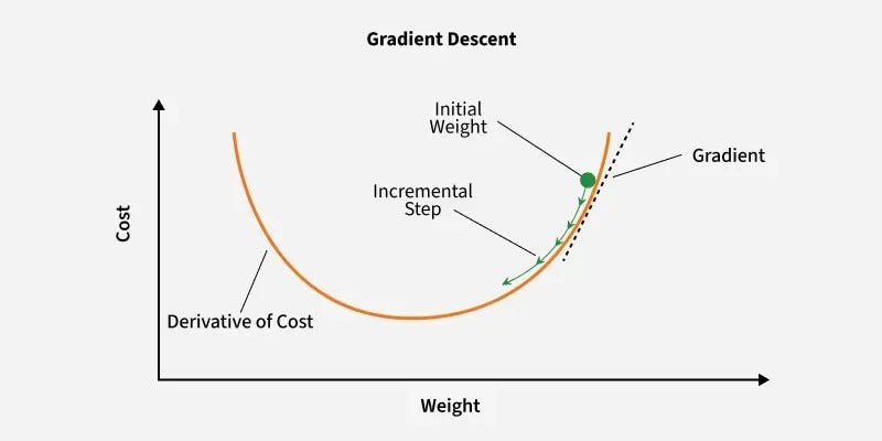
1️⃣ Gradient Descent (Batch GD)
Calculates the gradient of the cost function using the entire dataset for each iteration.
How it works: Updates weights using the entire dataset in one forward + backward pass per epoch.

Weight update:

Use case: Small datasets, resource-heavy systems.
What it lacked: 🚫 Resource-intensive — requires loading millions of records into RAM every epoch. If your dataset is large, this optimizer is practically unusable.
2️⃣ Stochastic Gradient Descent (SGD)
Calculates the gradient and updates parameters using only one training example per iteration.
How it works: Updates weights after processing one sample at a time. One epoch = million iterations (for 1M records).
What it solved: No need for massive RAM. Processes one record at a time.
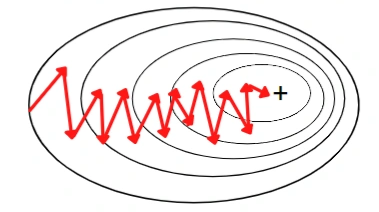
What it lacked: 🚫 Extremely noisy convergence — the loss curve zigzags wildly because each update is based on a single sample. 🚫 Slow convergence — time complexity is high. Takes 100M iterations for 100 epochs on 1M records!
3️⃣ Mini-Batch SGD
Splits the training dataset into small batches and performs updates for each batch.

How it works: A middle ground — processes batches of data (e.g., 1000 records) per iteration.
What it solved: Balanced resource usage + better convergence speed. For 1M records with batch size 1000 → only 1000 iterations per epoch.
What it lacked: 🚫 Still has noise — the zigzag movement is reduced compared to SGD but still exists. The path to global minima isn’t smooth.
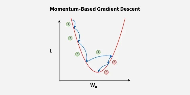
4️⃣ SGD with Momentum
It introduces a velocity term that accumulates the gradient of the loss function over time thereby smoothing the path taken by the parameters
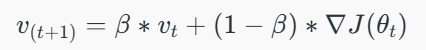
How it works: Introduces Exponential Moving Average (EMA) to smooth the gradient updates.
Instead of reacting to every single gradient spike, it considers past gradients with a weight β (typically 0.9).
Key formula:
Then, the model parameters are updated using:

What it solved: 🚀 Smoothed the convergence path — reduced noise, faster convergence, fewer oscillations. Think of it like a ball rolling down a hill with momentum — it doesn’t stop at every small bump.
Use case: Standard deep learning tasks where vanilla SGD struggles with noisy gradients.
5️⃣ Adagrad (Adaptive Gradient)
Adjusts the learning rate for each parameter individually, giving larger updates to infrequent features.
How it works: Makes the learning rate adaptive — it starts high and automatically decreases as we approach the global minima.

The denominator grows over time → learning rate shrinks.
What it solved: 🚀 No need to manually tune learning rate decay. Handles sparse features well.
What it lacked: 🚫 Learning rate can become too small too quickly, causing training to stop prematurely.
6️⃣ RMSProp
An improvement over AdaGrad that prevents the learning rate from shrinking too quickly by using a moving average of squared gradients.
How it works: Fixes Adagrad’s aggressive decay by using an exponential moving average of squared gradients instead of cumulative sum.

What it solved: Prevents the learning rate from vanishing completely — keeps training going even in later epochs.
Use case: Recurrent Neural Networks (RNNs), non-stationary objectives.
7️⃣ Adam (Adaptive Moment Estimation) — The Current Champion
The most popular choice today, combining the benefits of both Momentum and RMSProp for efficient and robust training.
How it works: Combines the best of both worlds — Momentum (first moment) + RMSProp (second moment).

Tracks both the mean and variance of gradients.
What it solved: Fast convergence, works well with noisy/stochastic objectives, requires minimal tuning.
Use case: Default choice for most deep learning applications today — CNNs, Transformers, GANs, you name it.
🎯 Key Takeaways:
Epoch = 1 forward + 1 backward pass through the data
Batch = Subset of data processed in one iteration
Iteration = One weight update step
(Example: 1,000 images with a batch size of 100 equals 10 iterations to complete 1 epoch)
The evolution of optimizers is a story of balancing memory efficiency, convergence speed, and stability.
Every new optimizer emerged because researchers found a flaw in the previous one — that’s how innovation happens. Find the loopholes, create something better.
Credits: Krish Naik https://www.youtube.com/live/GseZVPT-7dc?si=f7M7Hl8Petbb8Lv3 & GeeksforGeeks
Why Your Deep Learning Model Won't Converge — A Deep Dive into Optimizers was originally published in Towards AI on Medium, where people are continuing the conversation by highlighting and responding to this story.