A systems-level view of how long contexts shift LLM inference from compute-bound to memory-bound

You send a prompt to an LLM, and at first everything feels fast.
Short prompts return almost instantly, and even moderately long inputs do not seem to cause any noticeable delay. The system appears stable, predictable, almost indifferent to the amount of text you provide.
But this does not scale the way you might expect. As the prompt grows longer, latency does increase. But more importantly, the system itself starts behaving differently.
What makes this interesting is that nothing external has changed. The model and hardware is same. But the workload is not.
As sequence length grows, the way computation is structured changes.
The amount of data the model needs to access changes.
And the balance between computation and data movement begins to shift.
So the real question is not just why latency increases. It is:
What exactly is the model doing differently as the input gets longer?
If you are building or working with LLM systems, this behavior is not just a curiosity. It directly affects latency, cost, and ultimately how many users a system can serve reliably under load.
At a high level, the explanation is often simplified to:
Every token interacts with every other token.
But that description hides what actually matters.
The real issue is not just that these interactions exist.
It is how they scale with sequence length, and how they are executed on real hardware.
To understand why longer contexts change system behavior,
we need to look at what the model is actually computing when it processes a sequence.
Every Token Has a Question It’s Trying to Answer
It is tempting to think of a language model as reading text the way we do, moving left to right and gradually building an understanding of the sentence.
But that is not how the model operates.
Instead, for every token in the sequence, the model is trying to answer a specific question:
how much does each of the other tokens matter for understanding this one?
And importantly, this is not done one token at a time.
It happens for all tokens, in parallel, and is repeated across multiple layers of the model.
To make this concrete, consider a simple sentence:
The cat sat on the mat.
If the model is processing the token “sat”, it does not treat every other token equally.
“cat” is important because it tells you who is performing the action.
“mat” adds context about where the action is happening.
“The”, while necessary for structure, contributes very little meaning here.
So the model needs a way to weigh these tokens differently.
Now the question becomes: how does it actually do that?
The model does not rely on rules or grammar.
Instead, every token is represented as a dense vector of size d. These vectors are not just abstract representations. They are the actual data that must be moved through GPU memory during inference.
Each token is then projected into three components:
a Query representing what it is looking for
a Key representing what it contains
a Value representing the information it can contribute.
Now imagine the token “sat” comparing itself with every other token.
When it compares with “cat”, their representations tend to align in a way that reflects their relationship. The model has learned that subjects and actions are closely connected.
When it compares with “the”, this alignment is much weaker, since the word carries less semantic information in this context.
The model measures this alignment numerically using a dot product:
score(i, j) = Qᵢ · Kⱼ
You can think of this score as a measure of how relevant one token is to another.
But scores alone are not enough.
They need to be turned into weights.
This is done using a softmax function, which normalizes the scores so the model can focus more on relevant tokens and less on others.
These weights are then used to combine the Value vectors, producing a new representation for the token.
All of these steps are typically written together as:
Attention(Q, K, V) = softmax(QKᵀ / √d) · V
Rather than thinking of this as a formula to memorize, it helps to see it as a sequence of operations:
- compare tokens
- turn comparisons into weights
- use those weights to gather information
What makes this powerful is that every token participates in this process with every other token.
But this is also where the cost comes from. For a sequence of n tokens, this creates a dense pattern of interactions between all pairs of tokens.
And as the sequence grows, the number of these interactions grows rapidly.
This is the behavior that begins to dominate how the system runs.

Why the cost grows much faster than you expect
At this point, the mechanism of attention is clear.
Each token compares itself with every other token, producing scores that determine how information is combined.
What matters now is how this scales.
For a single token, the model compares it with all tokens in the sequence. If there are n tokens, that means n comparisons. And this happens for every token.
So the total number of comparisons becomes: n × n = n²
To put this into perspective
- 100 tokens → 10,000 comparisons
- 1000 tokens → 1,000,000 comparisons
But the real cost is not just the number of comparisons. It is what each comparison involves.
Each interaction is a dot product over vectors of size d, often thousands of dimensions wide.
So a million comparisons is not a million simple operations. It is billions of floating point multiplications, along with the need to repeatedly load these vectors from memory.
And this entire process is repeated across multiple layers of the model.
So a more realistic view of the cost looks like:
O(n² × d × L)
Where:
- n is the number of tokens
- d is the hidden dimension
- L is the number of layers
So, increasing the input length by 10x does not increase the work by 10x. It increases it by roughly 100x, and that increase is multiplied across every layer of the model.
To see why this becomes a real system constraint, consider very large sequence lengths.
An attention matrix for a sequence of 100K tokens has:
100,000 × 100,000 = 10¹⁰ entries.
Even in FP16, that is on the order of tens of gigabytes of memory just to store the attention scores. And this is only one part of the computation. Keys, Values, activations, and intermediate buffers all add to this footprint.
At this scale, the problem is no longer just more compute.
It becomes a question of whether the system can even hold this data,
and whether it can move it fast enough.
The Moment Inference Changes Its Character
Up to this point, everything we have described happens in a single forward pass.
The model processes the entire input together, using large, highly parallel operations. This phase is often referred to as prefill, where the model builds representations for the full prompt.
But this pattern does not continue.
Once the model starts generating new tokens, the computation changes fundamentally.
Because the model generates text one token at a time, each new token requires its own attention pass over everything that came before it.
What was previously a single, large, efficient computation becomes a sequence of smaller, repeated steps.
One step per token.
Each step depends on the entire history.
This is where the cost structure changes. The model is no longer doing one large computation.
It is performing many sequential computations, each growing slightly more expensive as the context expands.
And this loop is where the real cost of inference lives.
Why the Model Can’t Look Ahead
That sequential structure is not an implementation detail. It comes directly from how the model is trained.
In the previous section, we saw that once generation begins, the model produces one token at a time, and each step depends on everything that came before it.
But why is this constraint necessary?
If the model can attend to all tokens, why not also look at what comes next?
The answer lies in the task the model is trained to solve.
A language model is not trying to understand a sentence in full.
It is trying to predict the next token given what it has already seen.
For example, consider the sequence:
“The meeting starts at 10 and ends at”
At this point, the model must generate the next token, which might be “12”.
If the model were allowed to look ahead and see “12” during this step, the task would become trivial. Instead of learning patterns in language, it would simply copy the answer.
So the system enforces a strict constraint:
Each token can only attend to tokens that come before it.
This constraint is what we call causal attention.
In practice, it means that the model’s view of the sequence grows incrementally:
- the first token can only see itself
- the second token can see the first two
- the third token can see the first three
- and so on

So while attention is still dense, it is no longer symmetric across the sequence. Each token only has access to a prefix of the input.
To understand how this affects computation, consider the number of comparisons being made.
Instead of every token comparing with all n tokens,
the first token makes 1 comparison, the second makes 2, the third makes 3, and so on.
This gives:
1 + 2 + 3 + … + n = (n(n + 1)) / 2
This is smaller than n², but still grows quadratically with sequence length.
So while causal attention reduces the number of valid comparisons,
it does not fundamentally change how the system scales.
How context grows
Because of this constraint, the model builds context step by step.
At token 1, it has almost no context.
At token 10, it has a small amount of history.
At token 1000, it is carrying a large body of information that every new token depends on.
Each new token is not interpreted in isolation.
It is always interpreted in the context of everything that came before it.
And during generation, this context must be revisited at every step. For each new token, the model:
- forms a Query for the latest token
- comparing it against all previous Keys and Values
- produces a representation for just that token
Even though earlier tokens do not change, they remain part of every new step.
For example, if you are generating a 1000-token response:
- the first generated token attends to the prompt
- the second attends to the prompt + first token
- the third attends to the prompt + first two tokens
- the 1000th token attends to everything that came before it
So the amount of work grows with every step, not just because of attention itself, but because the context keeps expanding.
It’s Not a Compute Problem Anymore
The model is not just doing more work as the sequence grows. It is repeatedly operating over an ever-expanding history.
The cost is not coming from a single large computation.
It is coming from many sequential steps, each of which depends on all previous tokens.
That combination, growing context and repeated computation is what drives the real cost of inference, not just in theory, but in how systems behave under load.
And once you see that, the question becomes unavoidable:
If earlier tokens do not change, why are we processing them again at every step?
Where the real inefficiency comes from
In the previous section, we saw that during generation, the model repeatedly processes an ever-growing history.
At first glance, this suggests a clear inefficiency:
the model seems to be recomputing the same work again and again.
But modern LLMs do not actually work this way.
What KV cache actually does
In a naive implementation, every time a new token is generated, the model would recompute Keys and Values for all previous tokens and run the full attention computation again.
This would be prohibitively expensive. So modern LLMs avoid it.
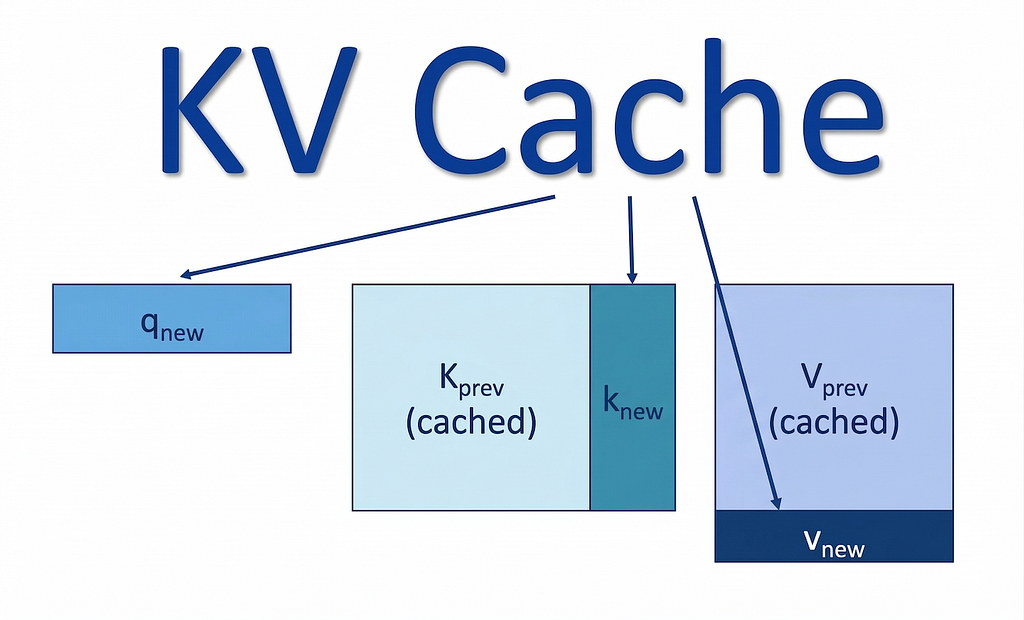
Instead, they use what is known as a KV cache.
The Keys and Values for past tokens are computed once, stored, and reused for every subsequent token. So when a new token is generated, the model does not rebuild the entire history. It only computes what is new.
The cost does not disappear. It moves.
Even though we avoid recomputation, the dependency on the full context does not disappear.
For every new token, the model must:
- form a new Query
- compare it against all previously stored Keys
- use those interactions to aggregate information from the corresponding Values
So while computation has been reduced, the model is still required to access the entire history at every step.
What this looks like in practice
Consider a single decode step at position 500.
The new Query is one vector. The Keys and Values it must attend over are 500 vectors.
Those vectors are already stored in GPU memory as part of the KV cache.
But they are not sitting in fast on-chip memory.
So for each step, they must be loaded from GPU memory into the compute units, used once for the attention computation, and then the process repeats.
At the next step, the model reads 501 vectors.
Then 502.
Then 503.
Nothing about the previous tokens changes. But they are still read again, step after step.
Earlier, during prompt processing, the system was dominated by large matrix multiplications, which GPUs handle efficiently.
During generation, the workload looks very different.
Instead of large, dense computations, the model performs many smaller operations that repeatedly fetch data from memory.
The real bottleneck
This is where the problem shifts.
Prefill is dominated by computation.
Decode is dominated by memory access.
More precisely, the limitation is not that the GPU stops working,
but that its compute units spend time waiting for data to arrive.
The bottleneck becomes memory bandwidth, not arithmetic.
This shift has clear consequences:
- GPU compute units sit idle waiting for memory transfers
- peak memory bandwidth becomes the ceiling on generation speed
- longer contexts increase per-token latency because more data must be fetched on every step
Even though each step is relatively small,
the repeated access to an ever-growing history becomes the dominant cost.
The deeper insight
KV cache does not eliminate the cost of long sequences. It transforms it.
From recomputing the past, to repeatedly reading the past.
And at scale, reading becomes the bottleneck.
KV cache trades a compute problem for a memory problem.
And whether that trade is beneficial depends entirely on how efficiently the system can move data.
Final takeaway
This shift is what defines modern LLM systems.
LLM inference does not slow down simply because models are large.
It slows down because of how tokens interact, and how those interactions evolve as the context grows.
At smaller context sizes, the system is dominated by computation.
Large matrix multiplications allow GPUs to process many interactions efficiently and in parallel.
But once generation begins, that structure breaks.
What was once a single, efficient computation becomes a loop, repeated once per token, where each step depends on everything that came before it.
And within that loop, the cost is no longer driven by arithmetic.
It is driven by memory access.
Every new token requires the model to reach back into its entire history, load what it needs, and use it just once before moving on.
This is the defining shift:
from compute-bound to memory-bound
KV cache makes this process feasible by avoiding recomputation.
But it does not remove the cost of long sequences.
It transforms it.
From recomputing the past,
to repeatedly reading the past.
And at scale, reading becomes the bottleneck.
Once you see this, the behavior of LLM systems becomes predictable:
- longer contexts increase per-token latency
- throughput drops under long-context workloads
- adding more compute does not linearly improve performance
Which leads to a more precise question:
If memory access is the bottleneck, how do modern systems structure, store, and retrieve this history efficiently?
Because solving that is not just an optimization. It is what makes large-scale LLM inference possible in practice.
Hope this gave you a clearer way to think about what’s really happening inside LLMs.
If it did, the next layer of the story, how systems actually manage this memory efficiently, becomes much more interesting.

Why LLM Inference Slows Down with Longer Contexts was originally published in Towards AI on Medium, where people are continuing the conversation by highlighting and responding to this story.