Why capture prices fall faster than market prices, how spatial correlation compounds the problem, and what portfolio-level decision architectures can do about it.
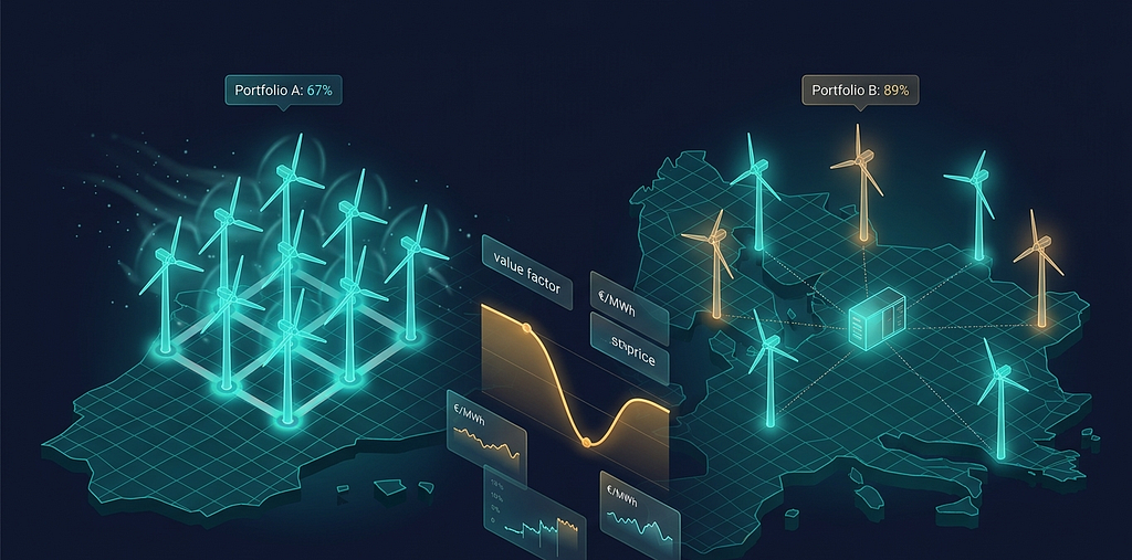
Two wind portfolios. Same total nameplate capacity — 500 MW. Same vintage of turbines. Same forecasting infrastructure.
Portfolio A is concentrated in Germany’s “belt of doom” — the central zone where, according to Pexapark, capture rates run roughly 20 percentage points below other parts of the country [1]. Portfolio B is diversified across regions with materially different weather regimes — Iberian solar-adjacent zones, the Nordics, and Italy, the latter described by S&P Global as a 2024 “bright spot” where capture prices comfortably exceeded breakeven [2].
Same MW. Same forecasts. Same operational excellence. A roughly 20-percentage-point gap in revenue per MWh, driven by where the assets sit on a map.
This article is about why that gap exists, why it is widening across European markets, and why closing it is a portfolio-level decision problem rather than an asset-level forecasting one.
Picking Up Where the Last Post Ended
The previous post argued that forecast distributions — not point estimates — should be the primary input to a trading policy. That argument was made at the asset level: a single wind farm, a single delivery hour, and a single decision.
Real renewable operators own portfolios and not a single asset. Portfolios with multiple sites, multiple technologies, and multiple bidding zones. And the most important uncertainty at the portfolio level is the dependence structure across assets.
Spatial correlation. Temporal correlation. Cross-technology correlation. These are the variables that determine whether a fleet’s risk can be diversified away or whether it compounds across the fleet on the worst days.
They are also the variables that determine capture price — the price at which a renewable portfolio actually sells its production, weighted by when production occurs.
This post is about putting those two ideas together: capture price erosion as a structural problem, and correlation structure as the lever that determines how badly any given portfolio is exposed to it.
What is Measured by the Capture Price
Capture price is straightforward in definition and treacherous in interpretation.
Formally, it is the production-weighted average market price a portfolio receives:
CP = Σ(P(t) × Q(t)) / Σ(Q(t))
Where P(t) is the day-ahead price at hour t and Q(t) is the portfolio’s production at that hour.
A portfolio’s revenue is not the average market price multiplied by total production. It is the correlated product of price and production, summed over time. If high-production hours coincide with high-price hours, the capture price exceeds the baseload. If high-production hours coincide with low-price hours, the capture price falls below it.
For dispatchable generation, capture price tends to exceed baseload — operators run when prices are high. For variable renewables, the relationship inverts. Wind and solar produce when conditions allow, not when prices reward production.
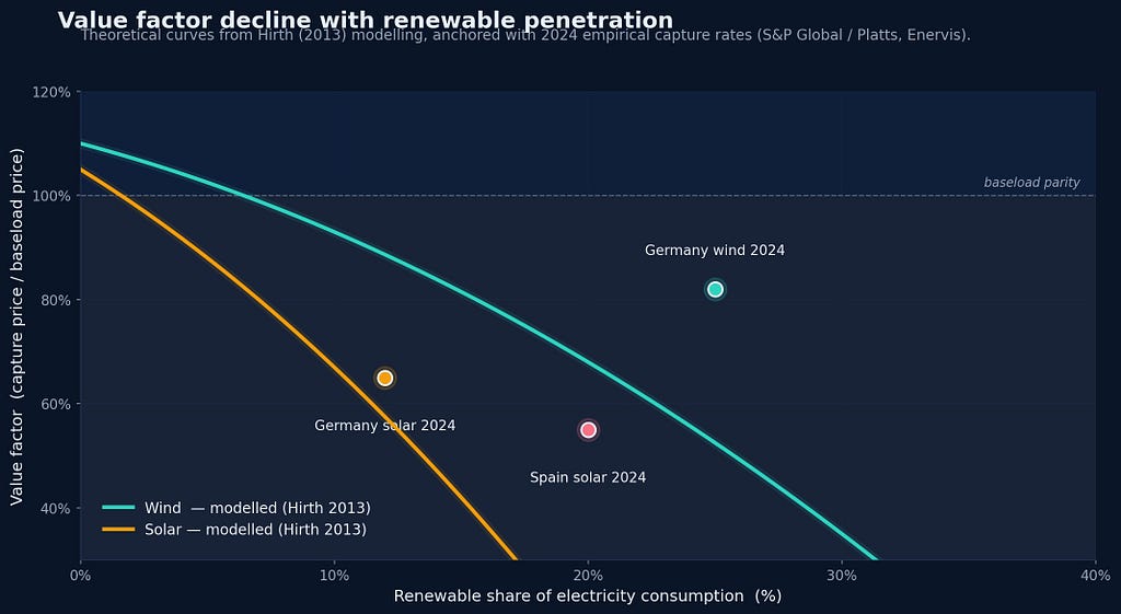
The ratio of the capture price to the time-weighted baseload price is the value factor, empirically formalized by Hirth [3] in the seminal study of variable renewables’ market value. A value factor of 1.0 means the portfolio captures the average price. A value factor below 1.0 — increasingly common for wind and solar in mature markets — means the portfolio is structurally selling into weakness. The broader argument that levelized cost (LCOE) systematically overvalues intermittent generation by ignoring this profile effect was first articulated by Joskow [4].
Empirical value factors have followed the trajectory the theory predicts. Hirth’s modeling for the European market estimates wind value factors falling from around 110% of the average power price at zero penetration to roughly 50–80% as wind penetration rises to 30% of total electricity consumption; for solar, similarly low values are reached already at around 15% penetration [3]. The contemporary German data tracks this: S&P Global / Platts assessed German onshore wind’s average capture rate at around 82% in 2024 (down some 20% from 2023), while German solar capture rates fell to roughly 60–70% over the same period [2]. Spanish solar collapsed further, to around 41% in April 2024 [5].
This decline is a structural feature of how wholesale electricity markets price simultaneous renewable production.
Why Capture Prices Fall Faster Than Market Prices
Two distinct mechanisms compound to push capture prices down.
The merit-order effect. Wind and solar bid at near-zero marginal cost. When they produce, they displace higher-marginal-cost generation in the merit order, suppressing the clearing price. The price reduction is largest precisely during hours of highest renewable output [6]. This is the cannibalization mechanism most often cited in the literature.
Self-cannibalization within the portfolio. A single wind farm faces market-wide cannibalization, but a portfolio also cannibalizes itself. When your ten wind farms produce simultaneously — because they sit under the same weather system — your own production contributes to the price suppression you experience. The bigger the portfolio, the larger the share of cannibalization that is your own doing.
Both mechanisms are driven by the same underlying variable: the correlation of production across the renewable fleet. When wind farms across a bidding zone produce in lockstep, prices collapse during high-output hours, and every operator captures lower prices. When production is decorrelated across geography or technology, the price suppression is smaller, and capture prices hold up.
This is why the same forecast quality, applied to the same MW of capacity, produces different revenue depending on where the assets sit — and why empirical analyses identify spatial and technological dependencies as primary drivers of value factor variation across Germany [7].
Spatial Correlation: The Hidden Driver
Operators often assume that geographic diversification reduces portfolio risk in proportion to the number of sites. The intuition borrows from financial portfolio theory: more uncorrelated assets, lower aggregate variance.
The intuition fails for renewables, because the assumption of low correlation rarely holds at the spatial scales where most operators concentrate.
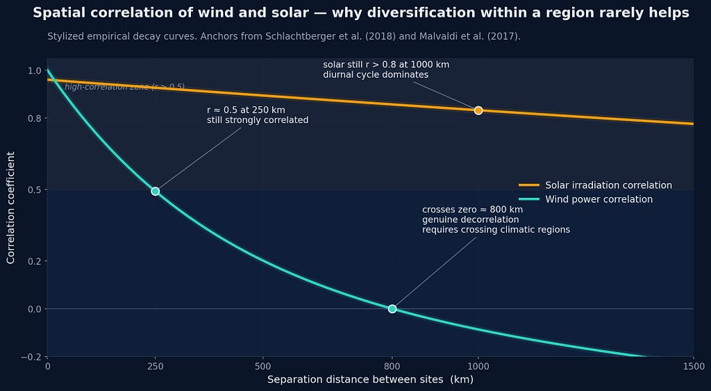
Wind production is driven by synoptic-scale weather systems — pressure patterns extending hundreds to thousands of kilometers. Empirical analyses of European wind data are consistent on the scale of this effect: wind generation patterns are strongly correlated within roughly 250 km, with correlation coefficients above 0.5, and the correlation only turns negative — making the sites genuinely complementary — at separations beyond about 800 km [8]. Country-level wind correlations across Europe routinely run in the 0.5–0.7 range even between distant pairs [9].
Solar correlation behaves differently but no less stubbornly. The diurnal cycle dominates: solar farms across an entire bidding zone produce at roughly the same hours, and empirical work shows solar irradiation correlations remaining above 0.8 even at separations of up to 1000 km [8]. Spatial spread within a single zone reduces variance modestly but does not change the fundamental fact that all solar in the zone produces at noon and none of it produces at midnight.
The implication is that “diversifying” a wind portfolio across, say, three German states often does very little for capture price. The farms remain under the same weather system most of the time. Real decorrelation requires crossing climatic regions — Iberia versus the North Sea, Nordic versus Continental — which introduces regulatory complexity, currency exposure, and grid connection challenges that make the diversification expensive even when it is meteorologically real.
The Joint Distribution Becomes the Risk
Article 3 made the case that decisions at the asset level depend on the shape of the forecast distribution. At the portfolio level, the equivalent claim is stronger: decisions depend on the joint distribution across assets, hours, and technologies.
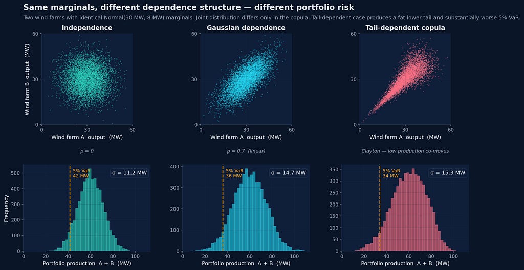
A portfolio whose marginal distributions look identical can have wildly different risk profiles depending on the dependence structure. Two examples:
Linear versus copula-driven dependence. Consider two wind farms with identical marginal forecasts — each predicted to deliver 30 MW with 8 MW standard deviation. Under independence, the portfolio variance is 128 MW²; the standard deviation is roughly 11 MW. Under perfect correlation, the variance is 256 MW²; the standard deviation is 16 MW. Under tail-dependent copulas — common when extreme weather affects both sites simultaneously — the joint distribution can produce tail risk substantially larger than either marginal would suggest [10].
Cross-technology dependence. Wind and solar are weakly anti-correlated within most European regions: high-pressure systems bring sun and reduce wind, frontal systems bring wind and reduce sun, and meteorological analyses find a “weak anticorrelation prevails” across the European domain at hourly resolution, with the effect strengthening seasonally [11]. This anti-correlation is not free risk reduction; it is bounded by the diurnal cycle (wind production is not strongly modulated by hour, while solar is) and by the fact that demand is also correlated with both. But for the purpose of portfolio capture price, even moderate anti-correlation between wind and solar within the same bidding zone substantially reduces self-cannibalization.
Capturing these effects in a forecast requires more than producing marginal distributions for each asset. It requires producing a coherent multivariate distribution — usually via ensemble methods that preserve scenario consistency, or through copula post-processing applied on top of marginal models [12]. A point forecast cannot represent this. Most production probabilistic forecasts also fail to represent it well, because they treat each asset’s distribution independently.
Portfolio Construction as a Decision Architecture
If capture price erosion is a structural feature of renewable markets, and if correlation structure determines a portfolio’s exposure to that erosion, then the question becomes: what can an operator actually do about it?
Three levers exist, and all three are decision-architecture questions, not forecasting questions.
Geographic allocation. When investing or contracting new capacity, the relevant question is not just “where is the resource good?” but “where does the resource decorrelate from the existing portfolio?” This is a portfolio-construction problem in the Markowitzian sense — but with renewable-specific constraints: grid connection availability, permitting, regional subsidy regimes, and PPA market depth. Optimal allocation requires a joint distribution model of production across candidate locations and a clear objective (capture price, value factor, revenue at risk).
Technology mix. Adding solar to a wind portfolio, or storage to a renewables portfolio, changes the joint distribution in structured ways. The decision is not just “build solar here” — it is “build solar that is anti-correlated with the wind we already own, in a regime where the combined production hits the merit-order curve at a different hour.” Hybrid portfolio optimization at the design stage is closer to a decision-architecture problem than to a feasibility study.
Operational dispatch. Even with capacity fixed, a portfolio with controllable elements (storage, curtailable assets, demand response) can shape its production profile to reduce capture-price exposure. This is where the policy architecture from the previous posts re-enters: storage dispatch, curtailment decisions, and bidding strategy across market stages all shift production from low-price hours toward higher-price hours. The mechanism by which a policy improves capture price is exactly the same mechanism by which it improves revenue per MWh in single-asset trading — but at the portfolio level, it must reason across assets, not just across stages.
These three levers operate on different timescales — investment decisions on years, contracting on quarters, dispatch on minutes — but they share a common requirement: a model of how production and price interact across the portfolio, conditional on weather, market, and grid state.
Where This Breaks Down in Practice
The principle is clean. The execution is hard for reasons worth naming.
Joint distributions are computationally and statistically expensive. Estimating a high-dimensional joint distribution across hours, sites, and technologies, conditioned on weather state and seasonality, demands far more data than estimating the marginals. Errors in the dependence structure can be larger than errors in the marginals, and they are harder to validate.
Capture price is a derived metric, not a directly forecastable one. It depends on the joint behavior of two stochastic processes — production and price — that are themselves correlated through the market mechanism. Forecasting capture price requires modeling both, plus the coupling between them. Decoupling the two for tractability gives wrong answers in exactly the regime that matters most: high-renewable, high-cannibalization periods.
Portfolio re-optimization is rare in practice. Most operators inherit their portfolio from historical investment decisions, PPA contracts, and acquisitions. Re-balancing the portfolio toward better correlation structure is constrained by what assets are available and at what price. The decision architecture often has to work with a suboptimal portfolio rather than redesign it.
Internal incentives are misaligned. Investment teams, asset management teams, and trading teams often optimize different objectives. Investment teams chase resource quality. Trading teams optimize within the portfolio they are given. The decisions that affect capture price most — geographic allocation, technology mix — are made upstream of the trading desk, often without joint-distribution modeling informing them.
This last point matters. The capture price problem is, in many organizations, structurally orphaned. The team with the data and tools to model it is downstream of the team making the decisions that determine it.
What Changes in the AI System
The shift from asset-level to portfolio-level decision architecture has concrete implications for how the underlying AI system is built.
The forecast must produce joint distributions across the full portfolio, not just per-asset distributions. This means ensemble-based or copula-based methods, not independent marginal models stitched together post-hoc.
The state representation must be portfolio-scoped. Position, asset availability, storage state, and forecast distributions need to be tracked at the level the policy operates on. A policy that decides per-asset dispatch without portfolio context will systematically misprice flexibility.
The objective function must include portfolio-level metrics. Capture price, value factor, and portfolio-level CVaR are the metrics that link operational decisions to commercial outcomes. Optimizing per-asset revenue and summing the results misses the cannibalization that occurs within the portfolio.
The simulation environment — for stochastic programming or RL — must reproduce the cannibalization mechanism. A simulator with exogenous prices does not capture self-cannibalization; the price process must respond to the portfolio’s own production for the policy to learn correctly.
None of this is exotic. It is the standard requirement for portfolio-level decision systems in adjacent domains (finance, supply chain, transportation). The energy industry is somewhat behind in adopting it, partly because the regulatory and market structures are recent enough that the data needed to estimate joint distributions has only become available at scale in the last decade.
Next in the series: “Market-Aware Maintenance: Aligning Asset Health with Price Regimes” — how outage scheduling, condition-based maintenance, and component replacement become trading decisions when the value of uptime varies systematically with market state.
This post is part of a series: AI Systems Architecture for Multi-Stage Electricity Markets.
References
[1] Pexapark. (2022). The Cannibalization Effect: Behind the Renewables’ Silent Risk. Industry report on capture rate variation across European markets, including the regional capture rate gap of approximately 20 percentage points within Germany.
[2] S&P Global Commodity Insights / Platts. (2025). Deflating capture prices pull solar, wind market values down across Europe in 2024 (and related Platts assessments). German onshore wind capture rate ≈ 82% (2024); Italian renewables identified as 2024 outperformer.
[3] Hirth, L. (2013). The market value of variable renewables: The effect of solar wind power variability on their relative price. Energy Economics, 38, 218–236.
[4] Joskow, P. L. (2011). Comparing the costs of intermittent and dispatchable electricity generating technologies. American Economic Review, 101(3), 238–241.
[5] Kpler / Enervis. (2024–2025). Spanish solar capture rate analysis — April 2024 monthly low of approximately 41%, with 2024 cumulative deflation across European markets.
[6] Sensfuß, F., Ragwitz, M., & Genoese, M. (2008). The merit-order effect: A detailed analysis of the price effect of renewable electricity generation on spot market prices in Germany. Energy Policy, 36(8), 3086–3094.
[7] Eising, M., Hobbie, H., & Möst, D. (2020). Future wind and solar power market values in Germany — Evidence of spatial and technological dependencies? Energy Economics, 86, 104638.
[8] Schlachtberger, D. P., Brown, T., Schäfer, M., Schramm, S., & Greiner, M. (2018). Cost optimal scenarios of a future highly renewable European electricity system: Exploring the influence of weather data, cost parameters and policy constraints. (Empirical correlation distances for wind and solar across European geographies).
[9] Malvaldi, A., Weiss, S., Infield, D., Browell, J., Leahy, P., & Foley, A. M. (2017). A spatial and temporal correlation analysis of aggregate wind power in an ideally interconnected Europe. Wind Energy, 20(8), 1315–1329.
[10] Papaefthymiou, G. & Kurowicka, D. (2009). Using copulas for modeling stochastic dependence in power system uncertainty analysis. IEEE Transactions on Power Systems, 24(1), 40–49.
[11] Monforti, F., Gaetani, M., & Vignati, E., et al. (2017). Local complementarity of wind and solar energy resources over Europe: An assessment study from a meteorological perspective. Journal of Applied Meteorology and Climatology, 56(1), 217–234.
[12] Pinson, P., Madsen, H., Nielsen, H. A., Papaefthymiou, G., & Klöckl, B. (2009). From probabilistic forecasts to statistical scenarios of short-term wind power production. Wind Energy, 12(1), 51–62.
Capture Price Risk and Spatial Correlation in Renewable Portfolios was originally published in Towards AI on Medium, where people are continuing the conversation by highlighting and responding to this story.