Every Rust ANN library I found had the same problem. None of them would let me change the distance function.
I’m building OmniPulse, a content fingerprinting system that uses Wavelet Scattering Transform to identify audio. I needed to search a large index of audio fingerprints by similarity. The fingerprints weren’t standard embedding vectors, but scattering coefficients and the most efficient way to compare them was Sliced-Wasserstein distance, not L2 or cosine. I went on a search to find the perfect Rust ANN Library.
Access this story for free here
The Problem With Existing Libraries
While searching, I came across some Libraries like instant-distance, hnsw_rs, and a few others. They’re good libraries. Fast, well-tested, production-grade. But all of them had one common issue, they all hardcoded their distance function. instant-distance takes Point types that implement its own Point trait with a fixed distance method. hnsw_rs is similar. If I had to use a custom metric like Sliced-Wasserstein, Hamming, a learned distance function or anything that isn’t L2 or cosine then I had to fork the crate or reimplement HNSW myself.
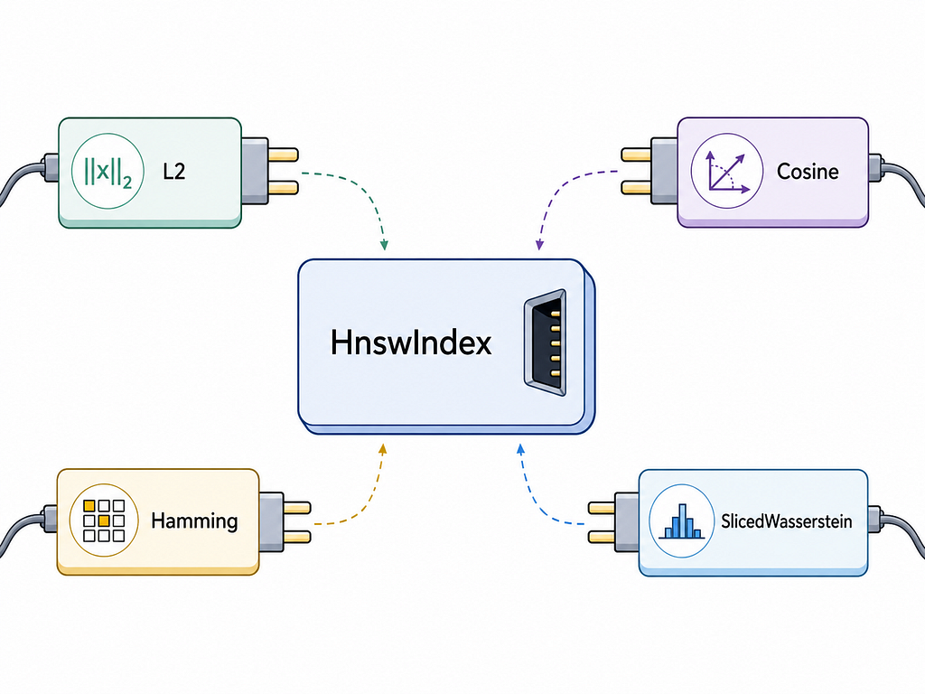
So, I choose to implement HNSW from scratch in Rust with a Metric trait that’s fully generic over the distance function. The index doesn’t care what metric you use. Plug in L2, cosine, Sliced-Wasserstein, or anything you implement the core algorithm is the same. The crate is vector-index, it’s on crates.io, and this post covers the design decisions, the algorithm, and when you should and shouldn’t reach for this crate.
What Is HNSW?
What does HNSW solve? Brute-force nearest neighbor search compares your query against every point in the index. For N=1M vectors at dim=128, that’s 128M multiplications per query. Even at a moderate scale this is too slow. HNSW (Hierarchical Navigable Small World) solves this with a graph-based index that answers “find the K nearest neighbors” in O(log N) time instead of O(N).
The core insight comes from small-world network theory. Build a graph where each node (vector) connects to its nearest neighbors. To find the nearest neighbors of a query, start at an entry point, greedily walk to whichever neighbor is closest to the query, repeat until you can’t get closer. This is fast but gets stuck in local optima on flat graphs.
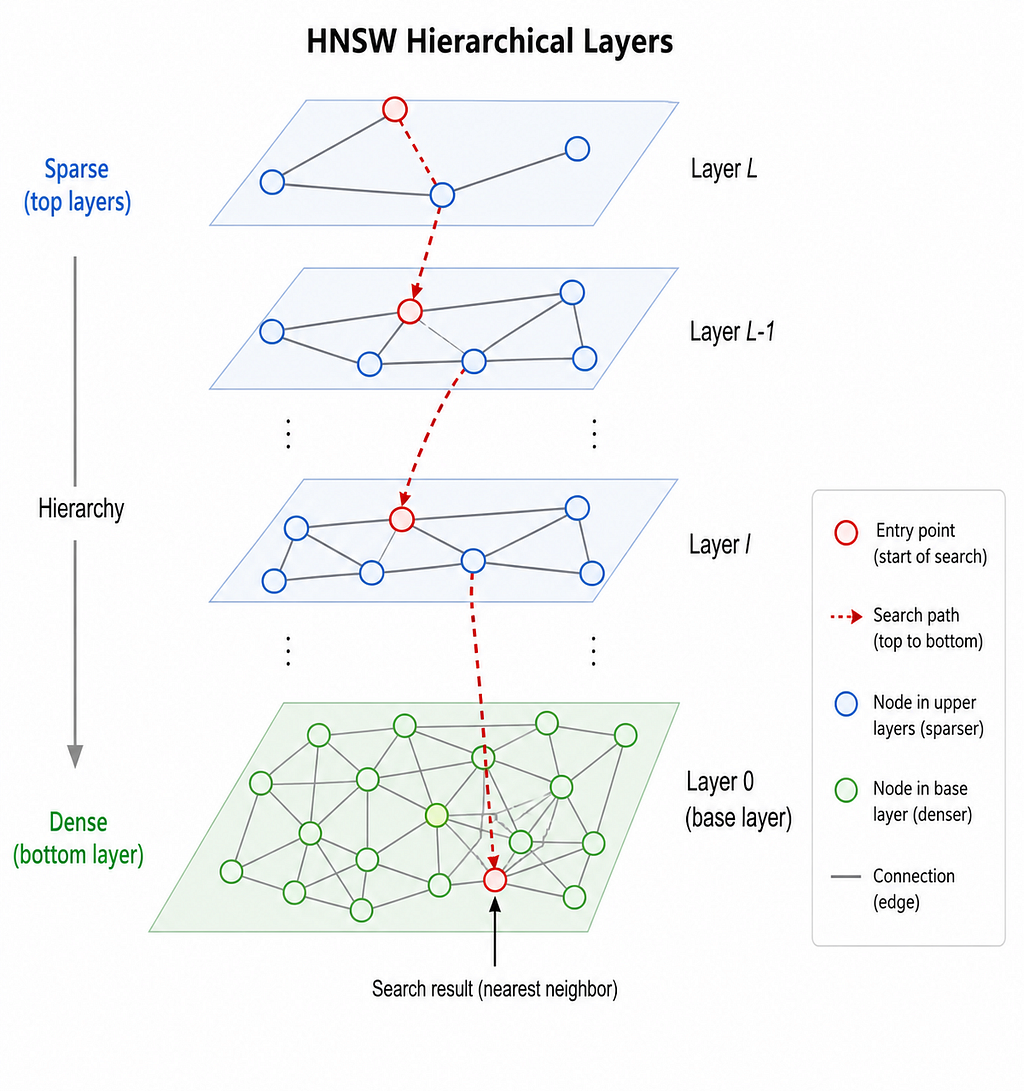
HNSW solves this with hierarchy. The top layer is sparse with only a few nodes, with long-range connections. Lower layers are progressively denser. Search starts at the top (fast, coarse navigation) and descends to the bottom (slow, precise). Same idea as a skip list, but in high-dimensional space.
Metric here works as a black box because at every step of the greedy walk, HNSW asks one question: “which of my neighbors is closest to the query?” That’s the only place the distance function appears. The graph structure, the hierarchy, the search algorithm and none of it cares what “closest” means. It just needs a number. This is why a generic Metric trait is the right abstraction. HNSW doesn’t know what Sliced-Wasserstein is. It just calls metric.distance(a, b) and gets a float back.
The Metric Trait
Let’s take a deep dive into this black box.
pub trait Metric {
    type Point;
    fn distance(&self, a: &Self::Point, b: &Self::Point) -> f32;
    fn dim(&self, point: &Self::Point) -> usize;
}
The trait has three parts. The associated type Point is what makes it generic — L2 uses Vec<f32>, SlicedWasserstein uses PointCloud. The distance method takes two points and returns an f32 — that's the only math the index ever does. And dim lives on the metric rather than the point type because for SlicedWasserstein, dimension is metric-specific.
The crate ships with L2 and Cosine built in. Here’s what L2 looks like under the hood — it’s the same trait:
pub struct L2;

impl Metric for L2 {
    type Point = Vec<f32>;
    fn distance(&self, a: &Vec<f32>, b: &Vec<f32>) -> f32 {
        a.iter().zip(b).map(|(x, y)| (x - y).powi(2)).sum::<f32>().sqrt()
    }
    fn dim(&self, point: &Vec<f32>) -> usize { point.len() }
}
No magic. If you can implement those two methods, you can use any distance function with the index.
Let’s see a simple example of distance function such as Hamming. It’s just three lines of code that implement this custom metric.
pub struct Hamming;
pub struct Hamming;

impl Metric for Hamming {
    type Point = Vec<u8>;

    fn distance(&self, a: &Vec<u8>, b: &Vec<u8>) -> f32 {
        a.iter()
            .zip(b.iter())
            .map(|(x, y)| (x ^ y).count_ones())
            .sum::<u32>() as f32
    }

    fn dim(&self, point: &Vec<u8>) -> usize {
        point.len() * 8
    }
}
That’s it. To use it with the index:
let mut index = HnswIndex::new(Hamming, HnswConfig::default());
index.insert(vec![0b10110011u8, 0b11001100u8]).unwrap();
index.insert(vec![0b10110001u8, 0b11001110u8]).unwrap();

let query = vec![0b10110011u8, 0b11001100u8];
let neighbors = index.search(&query, 1);
// returns the first vector at distance 0.0 — exact match
The index type is HnswIndex<Vec<u8>, Hamming>. The same index, the same search algorithm, only the metric changed. If you want to search for Sliced-Wasserstein tomorrow, you swap Hamming for SlicedWasserstein. The rest of your code doesn’t change.
All of these examples are in the crate’s test suite if you want to run them:
cargo add vector-index && cargo test
The DimensionMismatch error: The first vector inserted defines the dimension. Subsequent inserts that don’t match return IndexError::DimensionMismatch, it is a runtime check, not a compile-time one.
Algorithm 4: The Diversity Heuristic
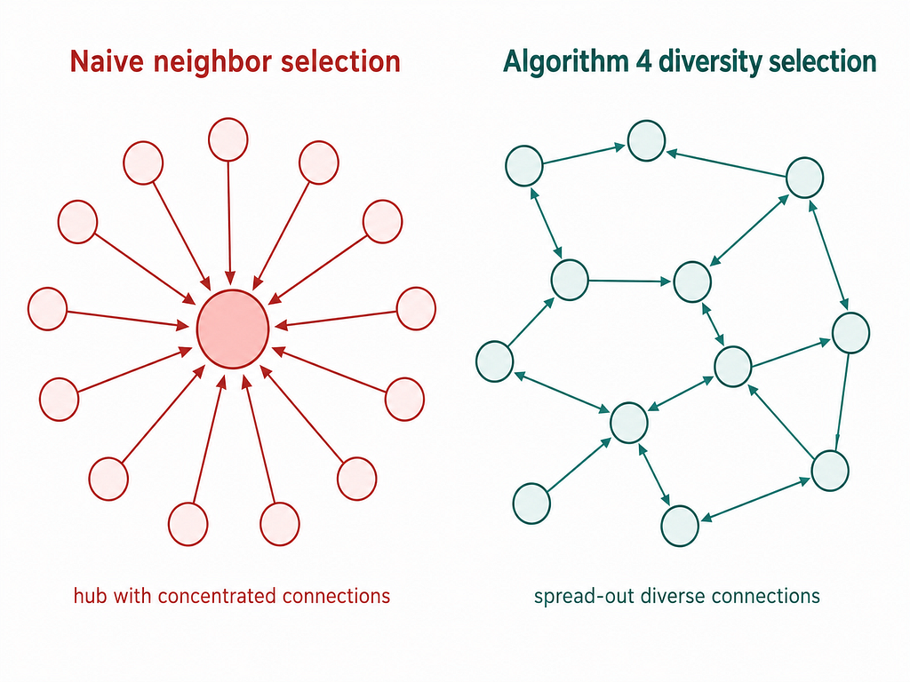
The greedy neighbor selection runs into an issue that when inserting a new node, the naive approach picks the M closest neighbors. This creates dense clusters and many nodes all pointing to the same popular hub. Search gets stuck because all paths lead to the same place.
A new algorithm suggested in the original HNSW paper (Malkov & Yashunin, 2018) which was a diversity heuristic. When selecting neighbors for a new node, instead of just picking the M closest, it checks: “does adding this neighbor actually improve coverage, or does it overlap with a neighbor I’ve already selected?” It keeps a neighbor only if it’s closer to the new node than to any already-selected neighbor. This preserves long-range connections and prevents the index from collapsing into cliques.
But there was one issue in this, if the diversity check is too aggressive, you end up with fewer than M neighbors and recall suffers. Algorithm 4 has a keep_pruned backfill which works if the diversity check discards candidates, the algorithm goes back and fills remaining slots from the discarded list, in ascending distance order. This is the part most implementations get wrong or skip. Getting it right is why recall holds up at high M values. But there is one trade-off as the diversity increases better recall at the cost of slower build time. The default HnswConfig is tuned for good recall on Gaussian data so for real world data with cluster structure may need different settings.
Let’s look at what 0.94 recall actually means.
Recall Validation
I ran the index against 5000 vectors and it returned the right neighbors 94% of the time. Specifically: for each query, I found the true 10 nearest neighbors by brute force, then checked how many HNSW returned. 0.94 means on average 9.4 out of 10 true neighbors were found
The benchmark setup.
The setup: 5000 random Gaussian vectors at dim=64, M=16, ef_construction=200, ef_search=50, k=10, averaged across 5 random seeds. Mean recall: 0.9410. Three honest caveats: this is synthetic data, recall scales with ef_search, and there’s no head-to-head comparison against instant-distance or hnsw_rs yet — that’s on the 0.2.0 roadmap.
Here’s the test setup if you want to reproduce it
#[test]
fn recall_benchmark() {
    let mut index = HnswIndex::new(L2, HnswConfig::default());
    for vec in &corpus {
        index.insert(vec.clone()).unwrap();
    }
    let results = index.search(&query, 10);
    // compare against brute force ground truth
    // mean recall across 5 seeds: 0.9410
}
The test is in the crate marked #[ignore] so it doesn’t run on every cargo test — run it with cargo test — ignored.
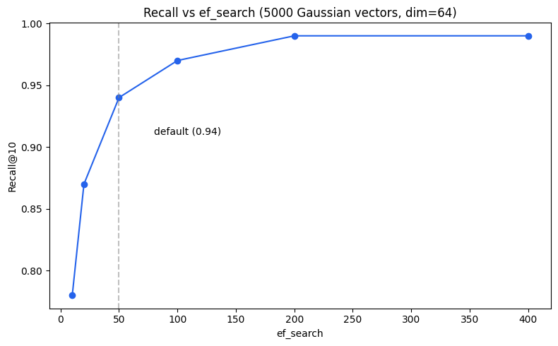
Three things worth knowing before you use these numbers. First, this is synthetic Gaussian data — real-world distributions with cluster structure or heavy tails will produce different recall. Second, recall scales directly with ef_search; the 0.94 number is at ef_search=50, and if you push it to 100 you’ll get closer to 0.97 at roughly double the query time. Third, there’s no head-to-head comparison against instant-distance or hnsw_rs yet — that benchmark is on the 0.2.0 roadmap.
For most retrieval workloads, 0.94 is the right trade-off. Increase ef_search if you need higher recall. Decrease it if you need faster queries and can accept 0.90.
Concurrent Access
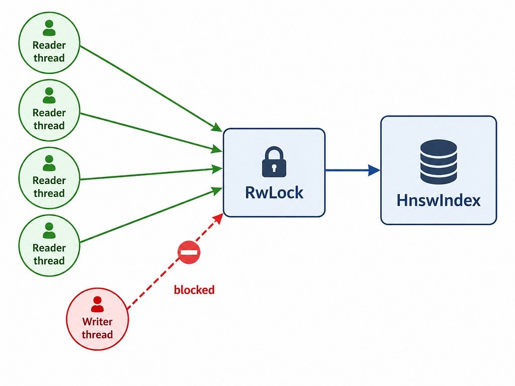
ConcurrentHnsw wraps HnswIndex in a parking_lot::RwLock that means many threads can search simultaneously. Writes (inserts) take an exclusive lock. This is the right pattern for a retrieval system where reads vastly outnumber writes, you’re building a corpus once, then querying it millions of times.
use std::sync::Arc;
use vector_index::{ConcurrentHnsw, HnswConfig, L2};

let index = Arc::new(ConcurrentHnsw::new(L2, HnswConfig::default()));

// Clone the Arc, share across threads
let index_clone = Arc::clone(&index);
tokio::spawn(async move {
    let neighbors = index_clone.search(&query, 10);
});
The main question is “Why parking_lot over std::sync::RwLock?”
The choice of parking_lot::RwLockcomes down to performance, it provides superior speed under contention and avoids the writer starvation issues found in some platform implementations of std. When you’re building a retrieval system that demands high read concurrency, these architectural details matter.
But there is one trade-off is this approach that is the write lock serializes all inserts. If you’re inserting thousands of vectors per second while serving queries, you’ll see lock contention. For batch-build-then-serve workloads this is fine. For high-frequency streaming inserts it’s a limitation worth knowing about.
When to Use It
Use it when you need a distance function that isn’t L2 or cosine like comparing point clouds, distributions, or anything where the geometric structure of the metric matters more than raw throughput. The abstraction is thin and the code is readable.
Don’t use it when you need maximum performance on standard embeddings — instant-distance and hnsw_rs are more battle-tested. Don’t use it if you need deletes or persistence. And if you’re at billion-scale, use Qdrant or Milvus.
What’s Missing in v0.1.0
v0.1.0 ships without delete support — HNSW deletion is non-trivial and getting it wrong destroys recall, so it’s deferred. No persistence either; the index is in-memory only, with bincode serialization planned for 0.2.0. The ef_search parameter is per-index, not per-query — a per-call override is coming. And no benchmarks against alternatives yet; the 0.94 number is on synthetic Gaussian data.”
In OmniPulse, this index runs with SlicedWasserstein as the metric for comparing scattering coefficient distributions of audio signals. The same code, the same algorithm, a different metric.
vector-index is on crates.io so download it and use it.
cargo add vector-index
The code is on GitHub at github.com/elli0t-yash/vector-index. If you have a use case that needs a custom metric, try it and file an issue if something doesn’t work the way you expect.
The next post covers sliced-wasserstein, which is the Optimal Transport metric that motivated building this crate in the first place. If you’ve ever needed to compare two distributions rather than two vectors, that one’s for you.
Building a Generic HNSW Index in Rust: When Cosine Distance Isn’t Enough was originally published in Towards AI on Medium, where people are continuing the conversation by highlighting and responding to this story.