Any enterprise deploying an AI support agent at scale, whether it is a telecom company handling billing queries, an e commerce platform managing returns, or an HR team answering policy questions, eventually runs into the same challenge within a few months. The agent goes live, user adoption increases rapidly, and then the infrastructure bill arrives.
Throughout this article, we will use a bank as our working example. Not because this problem is unique to banking — it absolutely is not — but because financial support queries are a clean, relatable illustration of what happens when thousands of users ask the same thing in a hundred different ways.
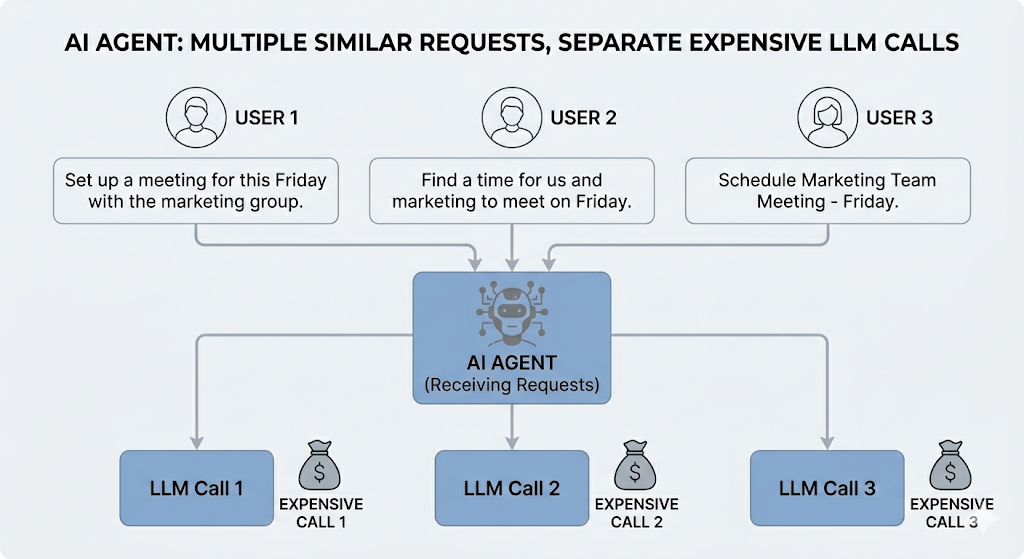
You dig into the logs and find something humbling: roughly 30 to 40 percent of queries coming into your LLM are asking the same things in different words. Not the same query. The same intent.
One user types “what’s the penalty if my EMI bounces?” Another asks “what happens if I miss my loan payment?” A third sends “will I get charged if my account doesn’t have enough funds on the due date?” Three users. Three LLM calls. One answer.
This is the problem semantic caching solves, and in enterprise AI deployments it is one of the highest-leverage optimizations you can make.
Why Traditional Caching Falls Apart Here
Traditional caching is exact-match. The cache key is the query string, and a hit only happens if someone types those exact words again.
cache["what is the minimum balance required"]
= "You need to maintain Rs. 10,000..."
# This misses:
# "how much should I keep in my account?"
# "minimum balance for savings account"
# "what balance do I need to avoid charges?"
In enterprise support scenarios, exact match hit rates hover around 2 to 5 percent. You cache thousands of responses and almost none of them get reused. The LLM gets called every single time.
What Semantic Caching Actually Does
Instead of matching strings, semantic caching matches meaning. Every incoming query gets converted into an embedding, which is a numerical vector that captures the semantic intent of the sentence. That vector is compared against previously cached query embeddings using cosine similarity.
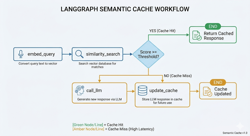
If the similarity score crosses a threshold (typically 0.75 or above), the cached response is returned without touching the LLM. If it falls below, the LLM gets called and the new query-response pair goes into the cache for next time.
Here is what that flow looks like:

The business implication is straightforward. You stop paying for inference on queries your system has already answered.
Building the Pipeline with LangGraph and Redis
LangGraph is a good fit here because semantic caching is not a single function call, it is a decision graph. You have branching logic, conditional LLM invocation, and state that flows between nodes.
The node structure looks like this:
Start with the shared state
Every node in a LangGraph pipeline reads from and writes to a shared state object. This is the backbone of the whole pipeline. Define it as a TypedDict so every node has a clear contract on what it receives and what it must return.
class CacheState(TypedDict):
    query: str                        # the raw user query, never mutated
    embedding: Optional[list]         # populated by embed_query, reused by update_cache
    cached_response: Optional[str]    # set only on a cache hit
    llm_response: Optional[str]       # set only on a cache miss
    cache_hit: bool                   # the routing flag that drives the conditional edge
cache_hit is the most important field here. It is the flag that LangGraph reads to decide whether to route toward END (serve the cached response) or forward to call_llm. Every other field is a data carrier.
Node 1: embed_query
def embed_query(state: CacheState) -> CacheState:
    response = client.embeddings.create(
        model="text-embedding-3-small",
        input=state["query"]
    )
    state["embedding"] = response.data[0].embedding
    return state
This converts the raw query string into a 1536-dimensional vector using OpenAI’s text-embedding-3-small. That vector is what gets compared against everything in the cache. The model is small, fast, and cheap -- a good fit for a step that runs on every single request.
Node 2: similarity_search
def similarity_search(state: CacheState) -> CacheState:
    query_vec = np.array(state["embedding"], dtype=np.float32).tobytes()
    results = r.execute_command(
        "FT.SEARCH", INDEX_NAME,
        "*=>[KNN 1 @embedding $vec AS score]",
        "PARAMS", "2", "vec", query_vec,
        "RETURN", "2", "response", "score",
        "DIALECT", "2"
    )
    if results[0] > 0:
        fields = results[2]
        result_dict = {}
        for i in range(1, len(fields), 2):
            key = fields[i - 1].decode() if isinstance(fields[i - 1], bytes) else fields[i - 1]
            result_dict[key] = fields[i]

        if "score" in result_dict and "response" in result_dict:
            # Redis returns cosine distance (lower = more similar).
            # Convert to similarity so the threshold reads intuitively:
            # SIMILARITY_THRESHOLD = 0.75 means "at least 75% semantically similar".
            similarity = 1 - float(result_dict["score"])
            if similarity >= SIMILARITY_THRESHOLD:
                state["cached_response"] = result_dict["response"].decode()
                state["cache_hit"] = True
                return state
    state["cache_hit"] = False
    return state
A few things worh understanding here. KNN 1 means we are asking Redis to return only the single most similar vector in the index. We do not need the top 5 or 10. We want the closest match and then we decide ourselves whether that match is good enough.
The distance vs similarity distinction matters here. Cosine similarity measures the angle between two embedding vectors. When two sentences mean the same thing, their vectors point in nearly the same direction — small angle, high cosine similarity. When two sentences are unrelated, their vectors point in different directions — larger angle, lower cosine similarity.
Mathematically: cos(0°) = 1 (identical direction, identical meaning) and cos(90°) = 0 (perpendicular, unrelated meaning).
Redis stores cosine distance, which is 1 - cosine similarity. This inverts the scale -- lower distance means more similar, which is the opposite of what you would intuitively expect from a variable called score.
Two examples to make this concrete:
Query:  "will I be charged if my EMI bounces?"
Cached: "what happens if my EMI bounces?"
Redis score (distance) : 0.05
Cosine similarity      : 1 - 0.05 = 0.95   → near identical meaning,
serve from cache
Query:  "how do I reset my net banking password?"
Cached: "what happens if my EMI bounces?"

Redis score (distance) : 0.72
Cosine similarity      : 1 - 0.72 = 0.28   → unrelated, call the LLM
So the conversion before the threshold check is:
similarity = 1 - score          # flip Redis distance back to intuitive similarity scale
if similarity >= SIMILARITY_THRESHOLD:
With SIMILARITY_THRESHOLD = 0.75, the check reads: "serve from cache only if the query is at least 75% semantically similar to a stored entry." That is far easier to reason about in production than a raw distance value where lower means better.
Node 3: call_llm (only on a miss)
def call_llm(state: CacheState) -> CacheState:
    response = client.chat.completions.create(
        model="gpt-4o",
        messages=[{"role": "user", "content": state["query"]}]
    )
    state["llm_response"] = response.choices[0].message.content
    return state
Nothing special here intentionally. This node only executes when the similarity search came back empty or below threshold. The routing logic (below) makes sure of that.
Node 4: update_cache
def update_cache(state: CacheState) -> CacheState:
    vec = np.array(state["embedding"], dtype=np.float32).tobytes()
    r.hset(f"cache:{state['query'][:50]}", mapping={
        "query": state["query"],
        "response": state["llm_response"],
        "embedding": vec
    })
    return state
We reuse the embedding already computed in embed_query rather than generating it again. The hash key uses the first 50 characters of the query as a human-readable prefix. This is fine for debugging but in production you would want a UUID or hash here to avoid key collisions on longer queries.
Wiring the graph
def route_after_search(state: CacheState) -> str:
    return "cache_hit" if state["cache_hit"] else "llm_call"

graph = StateGraph(CacheState)
graph.add_node("embed_query", embed_query)
graph.add_node("similarity_search", similarity_search)
graph.add_node("call_llm", call_llm)
graph.add_node("update_cache", update_cache)
graph.set_entry_point("embed_query")
graph.add_edge("embed_query", "similarity_search")
graph.add_conditional_edges("similarity_search", route_after_search, {
    "cache_hit": END,
    "llm_call": "call_llm"
})
graph.add_edge("call_llm", "update_cache")
graph.add_edge("update_cache", END)
pipeline = graph.compile()
add_conditional_edges is where LangGraph earns its place. The router function runs after similarity_search completes and returns a string key. That key maps to either END (cache hit path, response already in state) or "call_llm" (miss path). The graph handles the branching declaratively -- you are not writing if/else inside node functions, you are expressing the flow as a graph structure. That distinction matters when the pipeline grows more complex.
Redis vector schema
Before any of this runs, the index needs to exist:
from redis.commands.search.field import VectorField, TextField
from redis.commands.search.indexDefinition import IndexDefinition, IndexType

schema = [
    TextField("query"),
    TextField("response"),
    VectorField("embedding",
        "FLAT", {
            "TYPE": "FLOAT32",
            "DIM": 1536,           # must match the embedding model output dimension
            "DISTANCE_METRIC": "COSINE"
        }
    )
]
r.ft(INDEX_NAME).create_index(
    schema,
    definition=IndexDefinition(prefix=["cache:"], index_type=IndexType.HASH)
)
DIM: 1536 must match text-embedding-3-small exactly. If you switch embedding models, this number changes and you need to rebuild the index. FLAT is a brute-force index algorithm, which is fine for caches under roughly 100k entries. Beyond that, switch to HNSW for approximate nearest neighbor search at better speed.
Does It Actually Work? Benchmarks and Quality Evaluation
Before the numbers a quick note on scale. The benchmark below was run on a small controlled dataset of 15 queries across 5 intent categories. In a real enterprise deployment with thousands of daily users, messier query phrasing, and a much larger cache, the hit rate and cost savings will look different. The cold-to-warm comparison here is a best-case illustration of the mechanism working correctly.
With that context, here is what the pipeline produced:

91% latency improvement on a warm cache. The responses come back in under half a second consistently. That is the number users actually feel.
But latency is only half the story. The more interesting question is: when the cache returns a response, is it the right response?
Choosing the Right Similarity Threshold
This is where most teams get it wrong. They pick a threshold, ship it, and never look back. Then months later someone notices the cache is returning answers about minimum balance requirements in response to questions about transaction disputes — and they have no idea how long that has been happening.
The similarity threshold is the single most important tuning decision in a semantic cache. It controls the tradeoff between two things:
Precision — of the responses the cache serves, how many are actually correct for the intent of the query.
Recall — of all the queries that could have been served from cache, how many actually were.
Push the threshold too high and your cache barely fires — great precision, terrible recall, and you are paying for LLM calls you should not be making. Push it too low and the cache starts returning responses for queries that are superficially similar but semantically different — looks efficient on paper, silently wrong in production.
To make this concrete, take a single banking query:
Seed in cache: “what happens if my EMI bounces?”
Now imagine three different users send follow-up queries over the next hour:
Query A: “will I be penalised if my loan EMI fails?” Similarity score: 0.71. Same intent, different phrasing. This should hit the cache.
Query B: “what are the charges for closing my loan early?” Similarity score: 0.52. Related topic — loans — but different intent entirely. This should not hit the cache.
Query C: “can I get a waiver if my EMI bounced once?” Similarity score: 0.63. Edge case. Same topic, slightly different ask. Depending on how precise your cached answer is, this might be acceptable or it might mislead the user.
Now look at what happens as you move the threshold:

At 0.68 you get the safe hit — Query A, correct intent, no false positives. At 0.60 you pick up the edge case (Query C), which may or may not be acceptable. At 0.50 you start serving wrong answers for Query B. That is where precision collapses.
This is exactly why neither precision nor recall alone tells you enough. You need a single number that captures both — and that is where the F1 score comes in.
F1 score is the harmonic mean of precision and recall:
F1 = 2 × (Precision × Recall) / (Precision + Recall)
The harmonic mean is important here. Unlike a simple average, it punishes extreme imbalances. A cache with 100% precision and 0% recall gets an F1 of 0, not 50. A cache with 90% precision and 90% recall gets an F1 of 0.90. This makes F1 the right metric for threshold selection — it forces you to find a threshold that is actually good at both, not just dominant in one.

The relationship between precision, recall, and F1 as the threshold moves looks like this:
- As the threshold drops, recall rises steadily (more queries hit the cache).
- Precision stays flat until the threshold crosses into the “danger zone” where semantically different queries start matching, then it drops sharply.
- F1 peaks at the point just before precision starts to fall — that peak is your optimal threshold.
In practice, plot all three curves against threshold on your labeled dataset and look for the F1 peak. That is your starting point. Then shift it slightly upward if your domain is high-risk (compliance, legal, financial advice), or hold it at the peak if you are optimising purely for cache efficiency on general FAQ content.
The practical way to find your threshold is to build a small labeled dataset of 20 to 30 query pairs for your domain — a mix of true paraphrases and different-intent queries — run them through the pipeline, plot the similarity score distribution for each group, and pick the threshold that sits in the gap between the two clusters.
There is no universal right answer. The threshold is a product decision as much as an engineering one.
Hardening It for Production
A few things that matter once you move past a pilot:
TTL by topic category. Product information (loan rates, account types) changes quarterly. Regulatory disclosures change less often but matter more when they do. Policy information (fraud reporting timelines) can go stale overnight. Tag your cache entries by category and set TTL accordingly rather than using a single global expiry.
Query normalization before embedding. Users type with typos, abbreviations, and informal language. Running a lightweight normalization step before embedding (lowercasing, expanding contractions, correcting obvious misspellings) meaningfully improves hit rates without affecting quality.
Session-aware caching. A user mid-conversation asking “what are the charges?” means something different than a fresh session asking the same question. Consider including lightweight conversation context in the embedding input for agents handling multi-turn conversations.
Cache invalidation triggers. Wire your cache to your product change events. When a fee structure updates or a policy changes, you want stale cached responses flushed immediately rather than waiting on TTL.
The Bigger Picture
Most teams treat semantic caching as a performance optimization. That framing undersells it.
At enterprise scale, with thousands of concurrent users, semantic caching is what makes LLM-based support agents economically viable. It is the difference between a pilot that gets shut down because of infrastructure costs and a production system that scales.
The architecture is not complex. An embedding model, a vector store, a similarity threshold, and a branching graph. But getting the quality evaluation right, tuning the threshold per domain, and building the cache invalidation logic properly is what separates a demo from something you can actually run in production.
The full implementation with a benchmark notebook and sample banking dataset is on GitHub.
If you found this useful, follow for more on applied AI engineering and enterprise AI architecture.
Semantic Caching for Enterprise AI Agents: Cut Costs, Kill Latency was originally published in Towards AI on Medium, where people are continuing the conversation by highlighting and responding to this story.