A from-scratch PyTorch implementation, a head-to-head comparison with my MAE repo, and the three bugs that almost killed it.
78.97% vs 72.66%.
The first number is I-JEPA on STL-10 with a frozen encoder — a single linear layer trained on top of features that never updated. The second is my own MAE implementation on the same dataset, with the entire encoder fine-tuned for 15 epochs on labeled data.
Same backbone. Same dataset. Same pre-training budget. The frozen one wins.
That result is the reason this post exists.
A few months ago, I built a Masked Autoencoder from scratch and wrote about it here. MAE is the canonical “predict the missing pixels” self-supervised method, and it’s a great place to start. After I wrote about JEPA more broadly last month — Yann LeCun’s argument that AI should predict representations, not pixels — I kept thinking: that’s a beautiful idea, but does it actually buy you anything in practice?
So I built I-JEPA from scratch with the same backbone, the same dataset, and the same pre-training budget as my MAE — and ran them head-to-head.
This post is what I learned. The result. The architecture. The three bugs that took me days to find. And what the model actually sees when you look inside.
Repo: github.com/Alpsource/Visual-Representation-Learning-JEPA
The Question That Forced This Repo to Exist
Generative models predict pixels. JEPA predicts embeddings. That’s the one-line difference, and on paper it’s profound — pixel space is full of noise that doesn’t matter (textures, lighting, sensor grain), embedding space is supposed to throw all of that away and keep only what’s predictable.
But on paper is on paper. I wanted to see whether the gap held up under controlled conditions, on the same hardware, with no smuggled-in advantages on either side. So I matched everything I could:
- Same backbone — ViT-Base/16 at 224×224, built from scratch (no timm, no pre-trained weights)
- Same dataset — STL-10, 100k unlabeled images for pre-training, 5k labeled for evaluation
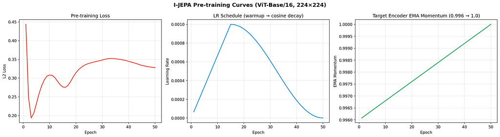
- Same pre-training budget — 50 epochs, AdamW, β=(0.9, 0.95)
- No augmentations during pre-training in either case
And then I gave I-JEPA the harder evaluation protocol on purpose. MAE got full fine-tuning — every weight in the encoder updated on labeled data. I-JEPA got a frozen encoder and a single linear probe. Linear probing is brutal: it cannot fix a bad representation, only read out a good one. If I-JEPA wins under that protocol, it’s a direct measurement of representation quality, not classifier capacity.
It won.

What I-JEPA Actually Does
If you read my JEPA primer post, skip this section. If you didn’t, here’s the 90-second version.
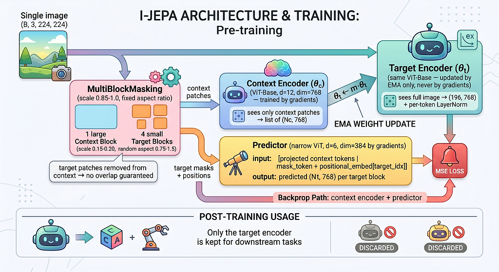
I-JEPA has three components. Two of them get thrown away after pre-training.
The context encoder is a ViT-Base that sees only a portion of the image — one large block covering 85–100% of the image, with target regions cut out. It produces a list of patch embeddings.
The predictor is a narrower ViT (depth 6, dim 384 — half the encoder’s width). It takes the context tokens, plus learnable mask tokens with positional embeddings telling it where the missing target blocks are, and outputs predicted embeddings for those targets. The narrowness is intentional: it forces the predictor to compress, not copy.
The target encoder is the secret. It’s a second ViT-Base — same architecture as the context encoder — that sees the full image and produces ground-truth embeddings for the target blocks. But here’s the twist: it never receives gradient updates. Its weights are an exponential moving average of the context encoder’s weights, drifting slowly toward whatever the context encoder is learning.
The loss is just the MSE between the predictor’s output and the target encoder’s output. No reconstruction. No contrastive pairs. No negatives. No hand-crafted augmentations. The model learns by trying to predict, in embedding space, what a slightly delayed version of itself would think the missing patches mean.
After pre-training, you throw the context encoder and the predictor away. You keep the target encoder, frozen. That’s your feature extractor.
The Masking Strategy Matters More Than You’d Think
I underestimated this.
MAE masks 75% of the image randomly, patch by patch. That’s a fine objective if you’re predicting pixels — you have to interpolate textures and edges, and you mostly succeed because adjacent pixels look like each other.
I-JEPA can’t get away with that. Random patch-level masking gives you a task that’s mostly local: most missing patches have visible neighbours, so the predictor can solve the problem with a kind of texture interpolation in feature space. That’s not what you want. You want the model to be forced to reason about object structure.
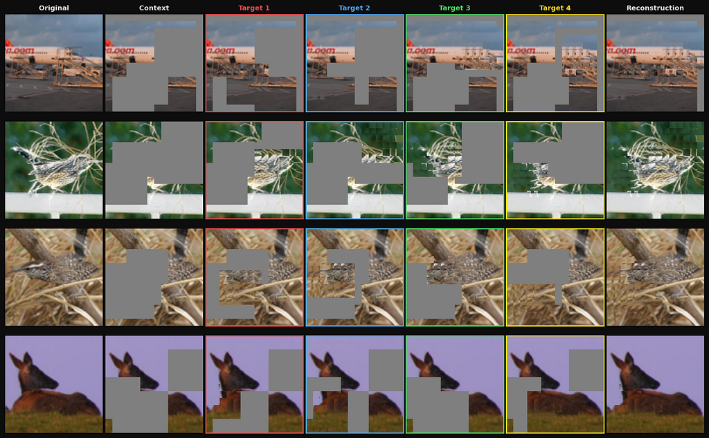
So I-JEPA masks four large target blocks per image — each one 15–20% of the image, with random aspect ratios. The context block covers 85–100% of the image, with the target regions surgically removed. The result is that the predictor frequently has to predict an entire object part — a wing, a wheel, a tail — from context that doesn’t include it.
You can see this in a single image:

The first time I ran this with MAE-style random masking by mistake, the loss curves looked beautiful and the linear probe accuracy was around 50%. The structured multi-block masking is the difference between a model that learns texture and a model that learns objects.
The Three Bugs That Almost Killed This
This is the section I would have wanted to read three weeks before I had it working.
JEPA-style models are notorious for failing silently. There’s no human-readable output to check (you’re predicting embeddings, not pixels — you can’t just look at a reconstruction and see something’s wrong). The loss can look reasonable while the model trains on garbage. Three specific bugs cost me days each. All three would have been invisible if I hadn’t been comparing to a known-good baseline.
Bug #1 — The attention mask that lied
When you batch images that produce variable numbers of context patches (which happens because the context block has a random scale and aspect ratio), you have to pad and provide an attention mask so the encoder ignores the padding. PyTorch’s scaled_dot_product_attention accepts a boolean attn_mask, and the convention is:
# True means: attend to this position.
attn_mask: Bool[B, num_heads, L_q, L_k]
Most padding mask conventions you’ll see in tutorials and in NLP libraries use the opposite:
# True means: this is padding, ignore it.
padding_mask: Bool[B, L]
I built my variable-length batching with the NLP convention and passed it straight to scaled_dot_product_attention without inverting. The encoder happily attended to all the zero-padded positions and ignored the real tokens.
The training loss looked fine. Slightly higher than expected, but not alarmingly so. The linear probe accuracy was 41%. I spent two days assuming the architecture was wrong before I dumped the post-attention activations and saw they were nearly identical for every input.
# What I had:
attn_mask = padding_mask                  # True = padding (wrong)
out = F.scaled_dot_product_attention(q, k, v, attn_mask=attn_mask)
# What I needed:
attn_mask = ~padding_mask                 # True = attend
out = F.scaled_dot_product_attention(q, k, v, attn_mask=attn_mask)
A single tilde. Two days.
Bug #2 — The loss that wasn’t a loss
The predictor outputs, per batch, roughly: 64 images × 4 target blocks × ~30 patches per block × 768 embedding dimensions ≈ 5.9 million scalar predictions.
If you sum the squared errors over all of those, you get a number around 50,000 at initialization. Beautiful. Looks like a loss.
It is not a loss.
Because the number of target patches varies from sample to sample (the random aspect ratios mean different blocks have different numbers of patches), the magnitude of .sum() fluctuates depending on which images happen to be in the batch. The gradient direction is meaningless — you're not minimizing a stable quantity, you're minimizing a number whose scale depends on how many patches the cropping happened to produce that step.
# What I had:
loss = ((pred - target.detach()) ** 2).sum()
# What I needed:
loss = ((pred - target.detach()) ** 2).mean()
.mean() gives a stable value around 1–2 at initialization that decays smoothly. .sum() gives a number that looks like a loss and isn't.
The symptom: training looked like it was converging, but the linear probe accuracy was random. I caught this one by comparing my MAE training curves (which were stable) to the I-JEPA curves (which had a kind of jaggedness I’d attributed to the EMA target encoder). It was the loss reduction.
Bug #3 — The warmup that swallowed the entire training run
I use gradient accumulation to fit larger effective batches in 24 GB of VRAM. With BATCH_SIZE = 64 and ACCUM_STEPS = 4, the effective batch is 256 — but there are still 64-sized forward/backward passes. Each forward/backward is a "batch step." Each optimizer.step() only happens every 4 batch steps.
The learning rate scheduler must step on optimizer steps, not batch steps. Otherwise, it advances four times faster than it should.
# Numbers for 50 epochs on STL-10:
batches_per_epoch     = 1562
optimizer_steps_per_epoch = 1562 // 4  =  390
total_optimizer_steps = 390 * 50  =  19,500
warmup_steps_intended = 390 * 15  =   5,850   # 15-epoch warmup
I had been computing warmup_steps and total_steps from raw batch counts: 1562 × 15 = 23,430 warmup steps, 1562 × 50 = 78,100 total. Then I was calling scheduler.step() once per batch.
Net effect: the warmup phase (23,430 scheduler steps) was longer than the actual number of optimizer steps in the entire 50-epoch training run (19,500). The learning rate was still ramping up when training ended. It never reached the peak value. The model had trained on a learning rate of roughly 5e-4 for 50 epochs instead of the schedule I designed.
# What I had:
scheduler.step()  # called every batch
warmup_steps = 15 * 1562
total_steps  = 50 * 1562
# What I needed:
if (batch_idx + 1) % ACCUM_STEPS == 0:
    optimizer.step()
    optimizer.zero_grad()
    scheduler.step()                         # only after optimizer.step()
warmup_steps = 15 * (1562 // ACCUM_STEPS)
total_steps  = 50 * (1562 // ACCUM_STEPS)
This one was the most painful, because the symptom was just “the model is mediocre.” 68% linear probe accuracy. Better than chance, worse than I expected. No obvious failure, just a quietly broken training run.
What It Looks Like When It Works
JEPA models don’t reconstruct pixels, so you can’t just look at a side-by-side and verify the model is doing something sensible. But there’s a clever indirect check.
After pre-training, build a gallery of patch features by running the target encoder on a held-out set of images and storing every patch embedding. Then, for a fresh image, run the predictor on the context and ask it for the embedding of each target patch. For each predicted embedding, retrieve the gallery patch whose target-encoder feature is cosine-nearest. Place that patch back into the original image at the target location.
The model has never seen the actual target pixels. It only ever produced an embedding. So if the nearest-neighbour patches look anything like what should be there — same object, same orientation, plausible structure — the predictor has learned something real about the world.

When I first generated this figure, I sat with it for about ten minutes. It’s not photorealistic — it’s not supposed to be — but you can see the model has learned that an airplane wing belongs to the right of an airplane fuselage, that a horse’s body has a particular structure, that backgrounds and foregrounds occupy distinct embedding regions. None of that was supervised. The model never saw a label.
You can also look at the structure of the feature space directly:
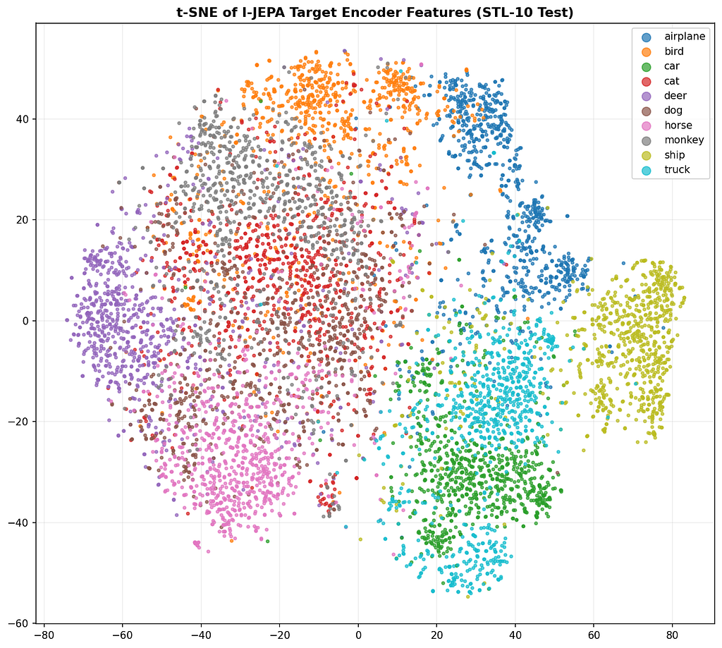
Ten clusters, ten classes, no labels involved in producing them. This is the part of self-supervised learning that still feels like magic to me even after building one from scratch.
The Result, In Detail
Linear probe on the frozen encoder, 5,000 labeled training images, 8,000 test images:
Method Evaluation Accuracy Macro F1 Random baseline Full fine-tune 46.19% — MAE (mine) Full fine-tune 72.66% — I-JEPA (mine) Frozen + linear probe 77.58% 77.42%
The 77.58% is the linear probe number. With a slightly stronger probing head, the same encoder reaches 78.97%, which is the headline number I led with.

What I’d Do Differently
If I were starting again, three things would change.
Pre-train longer. 50 epochs was a budget choice to keep the comparison fair against my MAE run. The original I-JEPA paper trains for hundreds of epochs and the linear probe number keeps climbing. The 78.97% I got is almost certainly a lower bound on what the architecture can do.
Try a larger pre-training set. STL-10 has 100k unlabeled images, which is small for self-supervised pre-training. ImageNet-1k pre-training on the same architecture would likely change the picture significantly — both for I-JEPA and MAE.
Add an entropy regularizer. I didn’t observe representation collapse during my runs, but I-JEPA models are known to be vulnerable to it, and the more recent literature (LeWorldModel, in particular) has shown that simple regularizers like a Gaussian prior on the latent distribution can stabilize JEPA training and reduce the number of fragile hyperparameters dramatically. That’s the next experiment.
Where This Is Going
This is the third post in what’s turned into a sequence. First came the MAE implementation — predict the pixels. Then came the JEPA primer — why predicting representations might be a better idea. This is the experiment that closes the loop.
What’s next on my end is the harder version of this question. I’m working on a JEPA-style architecture for drug-target interaction prediction as part of my PhD — same core idea (predict in embedding space, not in raw output space), different domain (proteins and small molecules instead of images). And in parallel, on the robotics side of my research, I’m building toward an action-conditional JEPA for visual-inertial odometry where the dynamicity of the scene is itself the JEPA prediction error. Both posts are going to take a while, but they’re coming.
If you want to follow that thread, the repo for this post is here:
github.com/Alpsource/Visual-Representation-Learning-JEPA
Everything is from scratch in PyTorch. The notebooks reproduce every figure in this post. The three bugs I just described are the ones I caught — there are almost certainly more I didn’t. If you find one, the issues tab is open.
Previous posts in this series:
- Why I Built a Masked Autoencoder (MAE) from Scratch (And How You Can Too)
- Beyond Tokens: How JEPA Is Quietly Teaching AI to Understand the World
I Built I-JEPA From Scratch and It Beat My Own MAE — With a Frozen Encoder was originally published in Towards AI on Medium, where people are continuing the conversation by highlighting and responding to this story.