Gradient descent is just the starting point — the real question is how fast and how reliably you can reach a good minimum.
The series has 4 parts:
- Part 1. Practical Aspects Improvements — https://pub.towardsai.net/improving-deep-neural-learning-networks-part-1-practical-approaches-and-applications-to-llms-72b8632e725b
- Part 2: Optimization Algorithms
- Part 3: Hyperparameter Tuning, Batch Normalization & Frameworks
- Part 4: From Deep Neural Networks to LLMs and Agentic AI
Let’s get into Part 2!
1. Mini-batch Gradient Descent
Mini-batch Gradient Descent sits between 2 extremes: Batch Gradient Descent (full batch) and Stochastic Gradient Descent (SGD).
- Batch Gradient Descent (full batch): uses the entire training set to compute the gradient before taking one update step.
for each epoch:
    gradient = compute_gradient(all m examples)
    update weights
This generates smooth and accurate gradient estimate, but runs extremely slow and requires the entire data set to be fit in memory, which could be impossible in many scenarios.
- Stochastic Gradient Descent (SGD): uses a single example at a time to compute the gradient and update weights.
for each epoch:
    for each example:
        gradient = compute_gradient(1 example)
        update weights
This method generates frequent updates with fast prgress, but extremely noisy and never really converges.
These two methods put mini-batch in the middle ground. Mini-batch splits the training set into small chunks of size t (typically 64, 128, 256, 512) and update weights after each chunk.
for each epoch:
  for each mini-batch of size t:
      gradient = compute_gradient(t examples)
      update weights
With 5,000,000 examples and batch size 1000, you get 5,000 weight updates per epoch instead of just 1. You make meaningful progress much faster.

Mini-batch cost is noisy step-to-step because each batch is a slightly different sample, but overall, trends move downward. This noise is actually a mild benefit as it helps escape shallow local minima.
Rules of thumb when choosing mini-batch size:
- Small dataset (< 2000 examples) — just use full batch, mini-batch has no advantage
- Larger datasets — typical sizes are 64, 128, 256, 512
- Make sure one mini-batch fits comfortably in CPU/GPU memory — if it doesn’t, you lose the hardware speed benefit entirely
2. Exponentially Weighted Averages
2.1. EWA Concept
Instead of taking a simple average of values, an exponentially weighted average (EWA) computes a running average that gives more weight to recent values and lets older values fade exponentially.
The formula is simply:
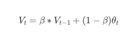
in which:
- Wₜ (or sometimes vₜ): the current average value
- β: hyperparameter that controls how much history to retain
- θₜ: current raw value (e.g: temperature, gradient,..)
Example: Using Paris temperature dataset, we can compare how EWA differs with different β.
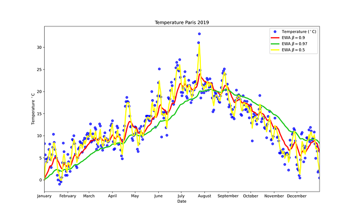
- β = 0.97: very smooth but also adapt very slowly
- β = 0.9: relatively balance
- β = 0.5: very responsive but extremely noisy
If you want to understand the meaning of the parameter β, you can think of the value

as the numbers of observations used to adapt your EWA.
For example, in this case, we can see that β = 0.9, n = 1/(1-0.9) = 10 => the average effectively covers the last 10 data points.

This is how we implement EWA:

2.2. Bias Correction in EWA
Problem: early in training, V_0 = 0 and there aren’t many past values to average over, so the EWA is systematically too low in the initial steps (v_1, v_2,..)
The fix is to divide by 1 − βᵗ at each step:

Early βᵗ is small, so (1- βᵗ) is small, making the correction large. As t grows, βᵗ -> 0, and the correction becomes ≈ 1, where it vanishes automatically once there’s enough history. Bias correction matters most in the first few steps of training.
EWA is the engine behind several important optimizers in deep learning: Gradient Momentum, RMSProp, and Adam.
3. Gradient Descent with Momentum
Standard Gradient Descent has a problem: as it updates weights using the raw gradient at each step. With mini-batches, those gradients are noisy, the update direction changes erratically from step to step, causing the optimizer to zigzag through the loss landscape instead of moving directly toward the minimum. This is especially bad in directions where the curvature is high.
This brings in Gradient Descent with Momentum. Momentum smooths out those erratic updates by maintaining a running average of past gradients, which are the exponentially weighted average explained earlier, and updating weights using that average instead of the raw gradient. It accumulates velocity in directions of consistent gradient and dampens oscillations in directions that keep switching size.

Momentum doesn’t change where you’re going, it changes how you get there. By accumulating velocity in consistent directions and canceling noise in oscillating directions, it lets gradient descent move faster and more directly toward the minimum. It’s one of the simplest and most universaly effective improvements over vanilla gradient descent.
4. RMSprop (Root Mean Square Propagation)
Even with momentum, gradient descent can oscillate badly when the loss landscape is elongated (stretched in one direction and narrow in another). The learning rate that is safe for the steep direction is too slow for the gentle direction. In this situation, we would benefit from a different effective learning rate for each parameter, which normally is aggressive where the gradient is small ad consistent, but cautious when it’s large and oscillating. And RMSprop can do the job very well.
Implement RMSprop:
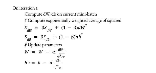
- Large S_dW → divide by large number → small effective step → slows down oscillating directions
- Small `S_dW` → divide by small number → large effective step → speeds up flat directions
5. Adam Optimization Algorithm
5.1 Adam
Adam combines both momentum and RMSProp. It maintains two running averages simultaneously — a smoothed gradient direction (momentum) and an adaptive per-parameter step size (RMSprop) — and uses both together to make each weight update. It’s the most widely used optimizer in deep learning because it inherits the benefits of both methods while being robust enough to work well across almost every architecture and problem type without heavy tuning.

Unlike standalone Momentum or RMSprop where bias correction is optional, Adam always applies it. Both V_dW and S_dW are initialized at zero, so early estimates are systematically too small. Since Adam divides by S_dW, an underestimated denominator inflates the update size, which makes the first few steps unreliably large. Bias correction fixes both terms simultaneously, making early training stable.
The numerator determines the direction, which is averaged and smoothed over recent gradients. The denominator scales each parameter’s step individually based on its gradient history. Together they produce updates that are both directionally stable and appropriately scaled per parameter.
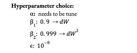
In practice, β₁, β₂, and ε are almost never changed from their defaults. The only hyperparameter that needs tuning is α. This makes Adam a practical advantages over vanilla SGD.
5.2. AdamW
The problem with Adam is that it folds weight decay into the gradient as a L2 regularization term to the loss function: L(θ) + (λ/2) * ||θ||^2, which affects the adaptive learning rates and hinder optimal convergence. This problem can be alleviated by AdamW, a smarter version of Adam, as it decouples weight decay from the gradient update step. Instead of adding weight decay to the loss function, it applies weight decay directly to the weights, making regularization and generalization more consistent.

### Adam L2 regularization ###

# compute gradients and moving_avg
gradients = grad_w + lamdba * w
Vdw = beta1 * Vdw + (1-beta1) * (gradients)
Sdw = beta2 * Sdw + (1-beta2) * np.square(gradients)
# update the parameters
w = w - learning_rate * ( Vdw/(np.sqrt(Sdw) + eps) )

### AdamW with direct weight decay method ##

# compute gradients and moving_avg
gradients = grad_w
Vdw = beta1 * Vdw + (1-beta1) * (gradients)
Sdw = beta2 * Sdw + (1-beta2) * np.square(gradients)
# update the parameters
w = w - learning_rate * ( Vdw/(np.sqrt(Sdw) + eps) ) - learning_rate * lamdba * w
A detailed example can be found in this Github project. With a significant improvement to Adam, AdamW is the standard optimizer for training LLMs (GPT, LLaMA), and many transformer models. At trillion-parameter scale, the adaptive per-parameter learning rates are critical because different parts of the network (embedding layers, attention heads, fead-forward blocks) have wildly different gradient magnitudes. A single global learning rate would be too large for some parameters and too small for others.

### PyTorch
# Adam
optimizer = torch.optim.Adam(
    model.parameters(),
    lr=1e-3,
    betas=(0.9, 0.999),   # β₁, β₂
    eps=1e-8)

# AdamW
optimizer = torch.optim.AdamW(
    model.parameters(),
    lr=1e-3,
    betas=(0.9, 0.999), # β₁, β₂
    eps=1e-8,
    weight_decay=0.01) #lambda
6. Learning Rate Decay
Recall the concept of learning rate:
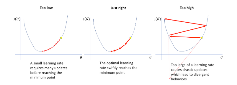
However, with a fixed learning rate, gradient descent faces a fundamental tension. A large learning rate makes early training fast, as the optimizer takes big steps and cover ground quickly. But near the minimum, those same big steps cause the optimizer to overshoot and oscillate around the solution rather than settling into it. A small learning rate converges precisely but wastes time crawling through the early stages of training. We would like to want both: fast early training, precise late converges. Learning Rate decay solves this by starting with a larger learning rate and systematically reducing it over time.
Some common decay schedules are Step Decay, Exponential Decay, and Cosine Annealing.
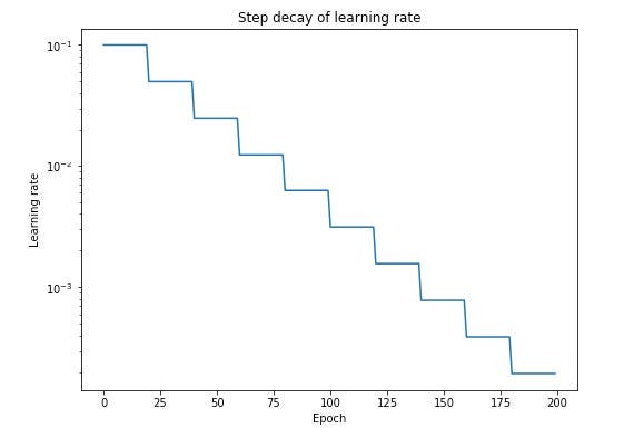
- Step Decay (Time-based decay)
Step Decay reduce learning rate by a fixed factor every few epochs. This is easy to implement and interpret, but it requires manual tuning of the decay factor and interval, making it less flexible than adaptive methods. This is often used as baseline, or used in classic ML and shallow networks.

- Exponential Decay: learning rate shrinks exponentially each epoch: aggressive, fast reduction.

where decay_rate < 1 (e.g: 0.95).
Used when we want the learning rate to drop sharply after a few epochs. Common in CNNs for image classification (ResNet, VGG-style training), or specific domains such as Physics/Chemistry (radioactive materials decay over time, reducing their mass by half at consistent intervals), Biology/Medicine (elimination of medication from the body; the rate of elimination often depends on the concentration remaining), Finance (fepreciation of assets, where the value of a house or car drops by a fixed percentage annually). Can decay too fast if decay_rate is set too aggressively.
- Staircase decay: set fixed drops every N steps is a discrete version of exponential decay. The learning rate stays constant for a fixed number of steps, then drops by a fixed factor, creating a staircase pattern.
This is method is common in training CNNs and classic deep learning pipelines (early ResNet papers used this). Simple to implement and reason about. Less smooth than cosine annealing but works well when you know roughly when the model plateaus.
- Inverse square root decay: Decays proportionally to 1/√t after warmup, which is slower than exponential but faster than time-based. Standard in original transformer training and still used in some NLP pipelines, though cosine annealing has largely replaced it in modern LLM training.

- Cosine Annealing: smoothly decays following a cosine curve. This is the most widely used schedule, ideal for deep neural network training and fine-tuning scenarios where finding the global minimum is difficult. It can be complex to turn the optimal T_max (cycle length) and restart frequency for specific dataset.
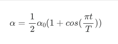
where: t is current step and T is total steps
This method is commonly used in Computer Visions (CNNs), Transformer and Language Modeling (LLMs), and scenarios requiring long training schedules.
Large models like transformers are unstable in the very first training steps as weights are randomly initialized and gradients are unreliable. Starting with a large learning rate immediately can cause the loss to explode early. The solution is linear warmup. We start with a very small learning rate and increase it linearly over the first few thousand steps, then decay from there.
# Model and Optimizer
model = nn.Linear(128, 10)
optimizer = torch.optim.AdamW(model.parameters(), lr=1e-3)

# schedule parameters
warmup_steps   = 1000
total_steps    = 10000
peak_lr        = 1e-3
min_lr         = 1e-6

# linear warm up + cosine decay scheduler
def warmup_cosine_schedule(step):
    if step < warmup_steps:
        # Linear warmup: scale from 0 → 1
        return step / warmup_steps
    else:
        # Cosine decay: scale from 1 → min_lr/peak_lr
        progress = (step - warmup_steps) / (total_steps - warmup_steps)
        cosine_decay = 0.5 * (1 + math.cos(math.pi * progress))
        # Scale to respect min_lr floor
        delta = min_lr / peak_lr
        return delta + (1 - delta) * cosine_decay

scheduler = LambdaLR(optimizer, lr_lambda=warmup_cosine_schedule)

# training loop
loss_fn = nn.CrossEntropyLoss()

for step in range(total_steps):
    # Dummy batch
    X = torch.randn(32, 128)
    y = torch.randint(0, 10, (32,))

    optimizer.zero_grad()
    loss = loss_fn(model(X), y)
    loss.backward()
    optimizer.step()
    scheduler.step()   # step scheduler every iteration, not every epoch

    if step % 1000 == 0:
        current_lr = scheduler.get_last_lr()[0]
        print(f"step {step:5d} | loss {loss.item():.4f} | lr {current_lr:.6f}")
Every major LLM training run uses warmup followed by cosine decay. The warmup prevents early instability from random initialization, and cosine decay ensures the optimizer is taking increasingly precise steps as the model converges. The learning rate schedule is considered one of the most important hyperparameters in LLM training. Getting it wrong can waste millions of dollars in compute.
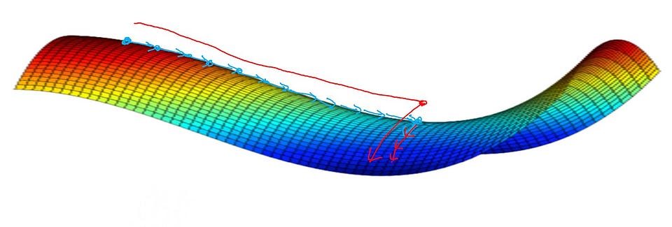
7. Problem of Local Optima
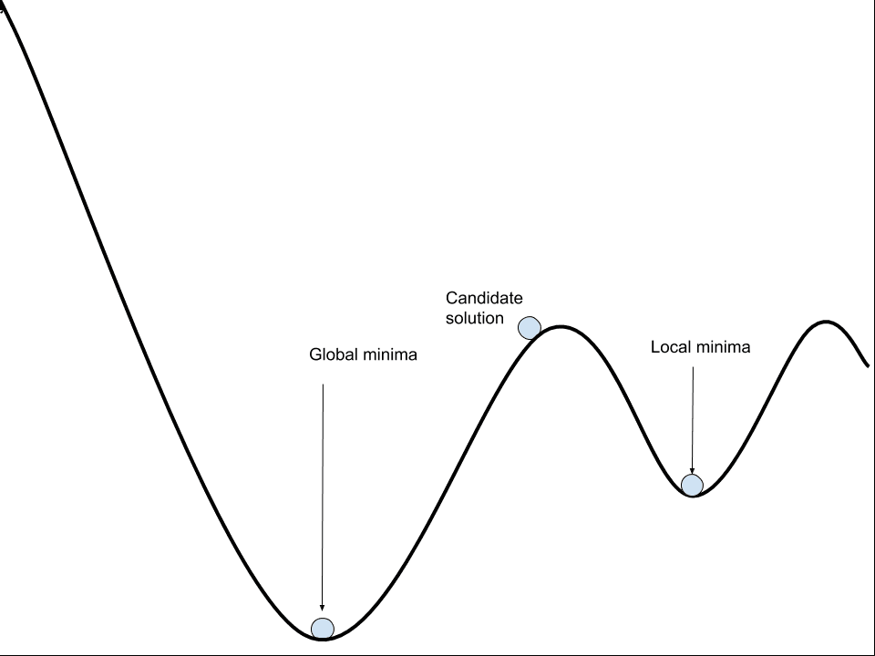
The classic fear in training neural networks was that gradient descent would get stuck in a local minimum and never get to a better solution (global minimum). This intuition comes from low-dimensional thinking: in 2D or 3D, local minima are easy to visualize and seem like a real trap.
However, it is mostly not a problem in deep learning. In a network with millions of parameters, a local minimum requires the loss surface to curve upward in every single dimension simultaneously at that point. The probability of that happening by chance is astronomically small. What you encounter instead at most critical points (where gradient = 0) are saddle points, which are points that are a minimum in some dimensions but a maximum in others.

In high-dimensional spaces, saddle points are exponentially more common than local minima. And crucially, saddle points are escapable, as the gradient is nonzero in most dimensions, so gradient descent naturally rolls away from them.
The real problem isn’t local minima, it’s plateaus: large flat regions of the loss landscape where gradients are very small but nonzero, and the optimizer crawls painfully slowly.
The optimizer isn’t trapped, it’s just moving very slowly because the gradient signal is weak. This is why:
- Momentum helps as it accumulates velocity through flat regions
- Adam helps as its adaptive learning rates take larger steps where gradients are small
- Learning rate warmup helps as ensures you enter the plateau with enough velocity to push through
The local optima problem as classically conceived is largely not the bottleneck in modern deep learning. The loss landscapes of large neural networks are high-dimensional enough that the optimizer almost always finds a path to a good solution. The practical challenges are plateaus, training instability, and getting through flat regions efficiently, which is exactly what momentum, Adam, and learning rate schedules are designed to address.
References:
[1] Exponentially Weighted Average, Tobías Chavarría on Medium, https://medium.com/@tobias-chc/exponentially-weighted-average-5eed00181a09
[2] Deep Learning Specialization: Courses by Andrew Ng on DeepLearning.AI
[3] Everything you need to know about Adam and RMSprop Optimizer, Sanghvirajit on Medium, https://medium.com/analytics-vidhya/a-complete-guide-to-adam-and-rmsprop-optimizer-75f4502d83be
[4] Understanding L2 regularization, Weight decay and AdamW, Another Deep Learning Blog, https://benihime91.github.io/blog/machinelearning/deeplearning/python3.x/tensorflow2.x/2020/10/08/adamW.html
[5] Adam vs. AdamW: Understanding Weight Decay and Its Impact on Model Performance, Ahmed Yassin, https://yassin01.medium.com/adam-vs-adamw-understanding-weight-decay-and-its-impact-on-model-performance-b7414f0af8a1
[6] Why is AdamW Often Superior to Adam with L2-Regularization in Practice?, GeeksforGeeks, https://www.geeksforgeeks.org/deep-learning/why-is-adamw-often-superior-to-adam-with-l2-regularization-in-practice/
[7] Neural Networks Learning Rate, Jeremy Jordan, https://www.jeremyjordan.me/nn-learning-rate/
Improving Deep Neural Learning Networks (Part 2): Optimization Algorithms was originally published in Towards AI on Medium, where people are continuing the conversation by highlighting and responding to this story.